Page 235 - Process Modelling and Simulation With Finite Element Methods

222 Process Modelling and Simulation with Finite Element Methods

with fully developed laminar Hagen-Poiseuille flow gives Ap=60. The fully
developed u-velocity profile is

24 = 6U,,,,Y (1- Y) (6.5)

Substitution into (6.2) yields the constant pressure gradient as -12 Urn,,,. Over
five unit lengths downstream, one would expect pinler=60Umean on the inflow
plane to achieve p=O at the outflow. So the additional pressure drop over
Hagen-Poiseuille flow is 0.463 (unitless due to scaling of viscosity and velocity).

Exercise 6.1
Refine the mesh and compute the additional pressure drop. Use the standard
refinement on the toolbar, and restart with the old solution as the initial guess.
Comment on the uniformity of the mesh and the variation in the additional
pressure drop. Is it worth refining the mesh yet again?
Now go to Draw Mode, and double click on the vertices at the bottom of the
notch. Edit them to place the orifice plate across to 40% blockage of the gap,
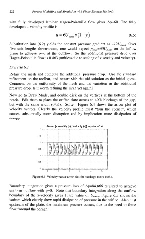
but with the same width (0.05). Solve. Figure 6.4 shows the arrow plot of
velocity vectors. Clearly the velocity profile must “turn the corner”, which
causes substantially more disruption and by implication more dissipation of
energy.

Arrow: [x velocity (u),y velocity (v)] epsilon=O 4
t
2 ’

ff
Figure 6.4 Velocity vector arrow plot for blockage factor &=0.4

Boundary integration gives a pressure loss of Ap=84.866 required to achieve
uniform outflow with p=O. Note that boundary integration along the outflow
boundary of the x-velocity gives 1, the value of U,,,,. Figure 6.5 shows the
isobars which clearly show rapid dissipation of pressure in the orifice. Also, just
upstream of the plate, the maximum pressure occurs, due to the need to force
flow “around the corner.”