Page 136 - Reliability and Maintainability of In service Pipelines

Case Studies on the Application of Structural Reliability 123

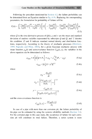
Following the procedure mentioned in Section 4.2, the failure probability can
be determined from an Equation similar to Eq. (4.9). Replacing the corresponding
parameters, the formulation for probability of failure will be:

( ! !)
ð t
Q
σ _ QjQ ðtÞ P o 2 μ ðtÞ μ _ QjQ ðtÞ μ _ QjQ ðtÞ μ _ QjQ ðtÞ
P f tðÞ 5 [ [2 1 Φ d τ
0 σ Q ðtÞ σ Q ðtÞ σ _ QjQ ðtÞ σ _ QjQ ðtÞ σ _ QjQ ðtÞ
ð5:3Þ
_
where Q is the time-derivative process of QðtÞ; μ and σ are the mean and standard
_
0
deviation of random variables represented by subscripts Q and Q, and ‘j denotes
the condition. [ and Φ indicate standard normal density and distribution func-
tions, respectively. According to the theory of stochastic processes (Melchers,
1999; Papoulis and Pillai, 2002), for a given Gaussian stochastic process with
mean function μ ðtÞ and autocovariance function C QQ ðt i ; t j Þ, the variables in the
Q
above equation can be determined as follows:

1 ρ
σ _ Q
_ ðP o 2 μ Þ ð5:4aÞ
μ _ QjQ 5 E QQ 5 P o 5 μ _ Q Q

σ Q
2 2 1=2
σ _ QjQ 5 ½σ _ Q ð12ρ ފ ð5:4bÞ
where
dμ ðtÞ
Q
5 ð5:4cÞ
μ _ Q
dt
" 1=2
2
5 @ C QQ ðt i ; t j Þ
σ _ Q : i5j ð5:4dÞ
@t i @t j
C ðt i ; t j Þ
Q _ Q
ð5:4eÞ
1=2
i
ρ 5 h

ð
C QQ t i ; t i Þ:C _ Q _ Q t j ; t j
and the cross-covariance function is:
@C QQ ðt i ; t j Þ

C Q _ Q t i ; t j 5 ð5:4fÞ
@t j
In case of a pipe with more than one corrosion pit, the failure probability of
the pipe can be estimated by using the systems reliability methods (Section 3.4).
For the corroded pipe in this case study, the occurrence of failure for each corro-
sion pit will constitute its total failure. Therefore, a series system is more