
Page 139 - Reliability and Maintainability of In service Pipelines
P. 139
126 Reliability and Maintainability of In-Service Pipelines
The randomness of the residual strength can be taken to account by introduc-
ing a random variable, ξ . This variable is defined in such a way that its mean is
Q
unity, i.e., E ξ 5 1 and its coefficient of variation, λ Q , is a constant. Thus,
Q
Eq. (5.13) can be expressed as:
QtðÞ 5 Q c tðÞ:ξ Q ð5:14Þ
where Q c ðtÞ is treated as a pure time function determined by residual strength
equation (e.g., Eq. (5.12)). The mean and autocovariance functions of QðtÞ are
(see, e.g., Li and Melchers, 2005)
μ tðÞ 5 E QtðÞ 5 Q c tðÞ E ξ
Q ½ Q 5 Q c tðÞ ð5:15Þ
2
C QQ t i ; t j 5 λ ρ Q c t i ðÞQ c ðt j Þ ð5:16Þ
Q Q
where ρ is autocorrelation coefficient for QtðÞ between two points in time t i and
Q
t j . With μ ðtÞ and C QQ t i ; t j , Eqs. (5.4a 5.4f) can be used to calculate other sta-
Q
tistical parameters of QðtÞ.
5.1.2 RESULTS AND ANALYSIS
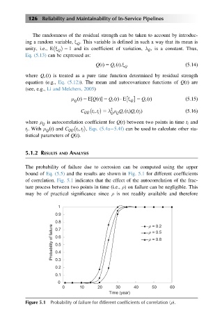
The probability of failure due to corrosion can be computed using the upper
bound of Eq. (5.5) and the results are shown in Fig. 5.1 for different coefficients
of correlation. Fig. 5.1 indicates that the effect of the autocorrelation of the frac-
ture process between two points in time (i.e., ρ) on failure can be negligible. This
may be of practical significance since ρ is not readily available and therefore
1
0.9
0.8 ρ = 0.2
Probability of failure 0.6 ρ = 0.5
0.7
ρ = 0.8
0.5
0.4
0.3
0.2
0.1
0
0 10 20 30 40 50 60
Time (year)
Figure 5.1 Probability of failure for different coefficients of correlation (ρ).