Page 141 - Reliability and Maintainability of In service Pipelines

128 Reliability and Maintainability of In-Service Pipelines

1
0.9
0.8
Probability of failure 0.6
0.7

0.5
0.4
Analytical (first passage
0.3
probability method)
0.2 Monte Carlo simulation method
0.1
0
0 10 20 30 40 50 60
Time (year)

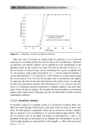
Figure 5.3 Probability of failure by different methods.

Since the costs of repairs are usually high for pipelines, it is of practical
importance to accurately predict the time for repairs for corroded pipes. Therefore
an optimum cost benefit analysis can be applied for asset management of the
pipeline system. In the current case study, the time for the pipe to fail, i.e., T f ,
due to fracture of corrosion pits, can be determined for a given acceptable risk
P a . For instance, using results presented in Fig. 5.3 for the analytical method, it
can be obtained that T f 5 19 years for P a 5 0:05. If there is no intervention during
the service period of (0, 19) years for the pipe, such as maintenance and repairs,
T f represents the time for the first intervention or the end of service for the pipe
for the given assessment criterion. The information of T f (i.e., time for interven-
tions) is of significant practical importance to pipeline engineers and asset man-
agers of the oil and gas industry. It can guide the decision makers in prioritizing
repairs and/or replacement of the pipes and also will help them to follow optimum
maintenance strategies.

5.1.2.1 Sensitivity Analysis

In reliability analysis of a pipeline system, it is of interest to indicate those vari-
ables that affect the pipe failure most so that more effort can focus on those vari-
ables. For this purpose, a parametric study can be carried out on three variables
that are deemed to be of significance to corrosion-induced pipe failures. These
are (i) corrosion rate for pit depth and length as represented by c d and c l ; (ii)
geometry of the pipe as represented by the diameter and wall thickness, D o and d;
and (iii) pipe property as represented by yield strength, σ y . The results are shown
in Figs. 5.4 5.6.