Page 138 - Reliability and Maintainability of In service Pipelines

Case Studies on the Application of Structural Reliability 125

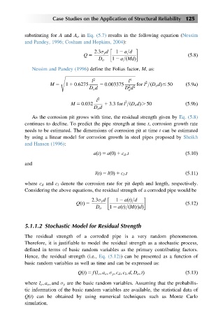
substituting for A and A o in Eq. (5.7) results in the following equation (Nessim
and Pandey, 1996; Cosham and Hopkins, 2004):
2:3σ y d 1 2 a=d
Q 5 ð5:8Þ
ð
D o 1 2 a= MdÞ
Nessim and Pandey (1996) define the Folias factor, M, as:
s ffiffiffiffiffiffiffiffiffiffiffiffiffiffiffiffiffiffiffiffiffiffiffiffiffiffiffiffiffiffiffiffiffiffiffiffiffiffiffiffiffiffiffiffiffiffiffiffiffiffiffiffiffiffiffiffiffiffiffiffiffiffiffiffiffi
l 2 l 4
2
M 5 1 1 0:6275 2 0:003375 for l = D o dð Þ# 50 ð5:9aÞ
2 2
D o d D d
o
l 2 2
M 5 0:032 1 3:3 for l = D o dð Þ. 50 ð5:9bÞ
D o d
As the corrosion pit grows with time, the residual strength given by Eq. (5.8)
continues to decline. To predict the pipe strength at time t, corrosion growth rate
needs to be estimated. The dimensions of corrosion pit at time t can be estimated
by using a linear model for corrosion growth in steel pipes proposed by Sheikh
and Hansen (1996):

atðÞ 5 a 0ðÞ 1 c d :t ð5:10Þ
and
ltðÞ 5 l 0ðÞ 1 c l :t ð5:11Þ

where c d and c l denote the corrosion rate for pit depth and length, respectively.
Considering the above equations, the residual strength of a corroded pipe would be

2:3σ y d 1 2 aðtÞ=d
QðtÞ 5 ð5:12Þ
ð
D o 1 2 aðtÞ= MðtÞdÞ
5.1.1.2 Stochastic Model for Residual Strength

The residual strength of a corroded pipe is a very random phenomenon.
Therefore, it is justifiable to model the residual strength as a stochastic process,
defined in terms of basic random variables as the primary contributing factors.
Hence, the residual strength (i.e., Eq. (5.12)) can be presented as a function of
basic random variables as well as time and can be expressed as:

QtðÞ 5 fðl o ; a o ; σ y ; c d ; c l ; d; D o ; tÞ ð5:13Þ
where l o ; a o ; and σ y are the basic random variables. Assuming that the probabilis-
tic information of the basic random variables are available, the statistical data of
QtðÞ can be obtained by using numerical techniques such as Monte Carlo
simulation.