Page 158 - Renewable Energy Devices and System with Simulations in MATLAB and ANSYS

Design of Residential Photovoltaic Systems 145

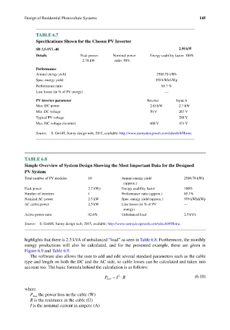
TABLE 6.7
Specifications Shown for the Chosen PV Inverter

SB 2.5-1VL-40 2.50 kW
Details Peak power: Nominal power Energy usability factor: 100%
2.70 kW ratio: 98%
Performance
Annual energy yield 2588.70 kWh
Spec. energy yield 959 kWh/kWp
Performance ratio 85.7 %
Line losses (in % of PV energy) —

PV inverter parameter Inverter Input A
Max. DC power 2.65 kW 2.7 kW
Min. DC voltage 50 V 267 V
Typical PV voltage 288 V
Max. DC voltage (inverter) 600 V 431 V

Source: S. GmbH, Sunny design web, 2015, available: http://www.sunnydesignweb.com/sdweb/#/Home.

TABLE 6.8
Simple Overview of System Design Showing the Most Important Data for the Designed
PV System
Total number of PV modules 10 Annual energy yield 2588.70 kWh
(approx.)
Peak power 2.7 kWp Energy usability factor 100%
Number of inverters 1 Performance ratio (approx.) 85.7%
Nominal AC power 2.5 kW Spec. energy yield (approx.) 959 kWh/kWp
AC active power 2.5 kW Line losses (in % of PV —
energy)
Active power ratio 92.6% Unbalanced load 2.5 kVA
Source: S. GmbH, Sunny design web, 2015, available: http://www.sunnydesignweb.com/sdweb/#/Home.

highlights that there is 2.5 kVA of unbalanced “load” as seen in Table 6.8. Furthermore, the monthly
energy productions will also be calculated, and for the presented example, these are given in
Figure 6.9 and Table 6.9.
The software also allows the user to add and edit several standard parameters such as the cable
type and length on both the DC and the AC side, so cable losses can be calculated and taken into
account too. The basic formula behind the calculation is as follows:

2
P loss = I ⋅ R (6.10)
where
P the power loss in the cable (W)
loss
R is the resistance in the cable (Ω)
I is the nominal current in ampere (A)