Page 242 - Renewable Energy Devices and System with Simulations in MATLAB and ANSYS

Electric Generators and their Control for Large Wind Turbines 229

relatively large air gap, the absence of PMs or brushes, and good utilization of the active material as
all phases are active simultaneously [28].
The following will be discussed:

• Optimal design of a surface PM rotor PMSG (8 MW, 3.2 kV, 480 rpm)
• Advanced control aspects of PMSGs with an AC–DC–AC converter connected to the grid

9.4.2 Optimal Design of PMSGs
Optimal design algorithms (ODAs) have to search for a set of parameters (variables) grouped in
X
a vector X, which minimizes (or maximizes) an objective (or fitting or cost) function F ob () and
fulfills some constraints.
The ODA presupposes

• A set of specifications, say, for the PMSG
• A model for the object (PMSG), analytical or (and) numerical, which links the parameters
(variables) to the objective (fitting) function
• A mathematical optimization (search) method that investigates part of the parameter vector
space (range), to yield with high probability a global optimum solution, within a reasonable
computational time

ODAs may be in general deterministic or metaheuristic (evolutionary) [19, 20]. Some of the
metaheuristic methods are enumerated here:

• Black hole–based optimization (BHBO)
• Particle swarm optimization (PSO)
• Gravitational search algorithm (GSA)
• Particle swarm optimization gravitational search algorithm (PSOGSA)

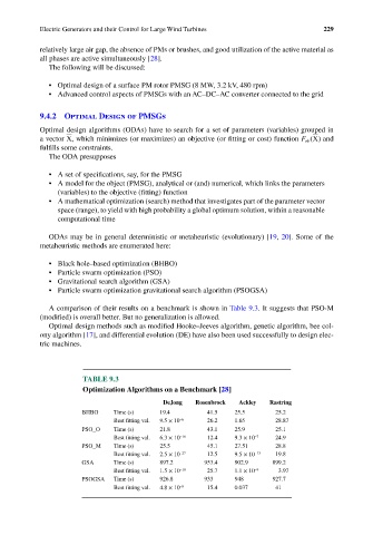
A comparison of their results on a benchmark is shown in Table 9.3. It suggests that PSO-M
(modified) is overall better. But no generalization is allowed.
Optimal design methods such as modified Hooke–Jeeves algorithm, genetic algorithm, bee col-
ony algorithm [17], and differential evolution (DE) have also been used successfully to design elec-
tric machines.

TABLE 9.3
Optimization Algorithms on a Benchmark [28]
DeJong Rosenbrock Ackley Rastring
BHBO Time (s) 19.4 41.5 25.5 25.2
Best fitting val. 9.5 × 10 −6 26.2 1.65 28.87
PSO_O Time (s) 21.8 43.1 25.9 25.1
Best fitting val. 6.3 × 10 −16 12.4 9.3 × 10 −7 24.9
PSO_M Time (s) 25.5 45.1 27.51 28.8
Best fitting val. 2.5 × 10 −27 12.5 9.5 × 10 −13 19.8
GSA Time (s) 897.2 953.4 902.9 899.2
Best fitting val. 1.5 × 10 −18 25.7 1.1 × 10 −9 3.97
PSOGSA Time (s) 926.8 933 948 927.7
Best fitting val. 4.8 × 10 −8 15.4 0.037 41