Page 237 - Renewable Energy Devices and System with Simulations in MATLAB and ANSYS

224 Renewable Energy Devices and Systems with Simulations in MATLAB and ANSYS ®
®

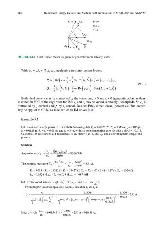
jω ψ R i P <0
s
s s
1 s
Q >0
s
S<0
V s
i d L i
d d
jL i
q q
ji q ψ
i s s
FIGURE 9.13 CRIG space phasor diagram for generator mode (steady state).

With ψ s = Li jL scq i and neglecting the stator copper losses,
s d +
3 * 3 s ( ) 3
*
VI s =
P s ≈ Re ( ) ω 1 Im ψ I s = 1 ω ( L s − L sc) i i q
s
d
2 2 2 (9.21)
(
3 * 3 *
VI s =
Q s = Im ( ) ) 1 ω Re ( ) = 3ω L i 2 + L i 2 )
ψ I
s
s
2 2 s 1 sd sc q
Both ideal powers may be controlled by the variation i > 0 and i < 0 (generating), but as dem-
d
q
onstrated in FOC of the cage rotor for IMs, i and i may be varied separately (decoupled). So P is
d
s
q
controlled by i control and Q by i control. Besides FOC, direct torque (power) and flux control
q
s
d
may be applied to CRIG as done earlier for IM drives [16].
Example 9.2
Let us consider a large power CRIG with the following data V n = 3200 V (Y), S n = 3 MVA, r s = 0.015 pu,
r r = 0.0125 pu, l sl = l rl = 0.05 pu, and l m = 3 pu, with six poles generating at 50 Hz with a slip S = −0.015.
Calculate the resistances and reactances in Ω, stator flux, i d and i q , and electromagnetic torque and
powers.
Solution
Approximately ψ s ≈ s V = 3200 2 / 3 = 8 306 Wb. .
π
ω 1 250
3 3200 2
The nominal reactance X n = V l n = V l n = 6 = .341Ω.
×
I n S n 310
Ω
×
Ω
=
Ω
Ω
.
R s = 0 015 × X n = 0 0512 , R r = 0 0427 , X sl = X rl = 05 3410 17 , X m =10024 ,
.
.
.
.
.
.
L m = 0 0326 , L s =H L r = 0 033 , L sc =H 1 087 mH
.
.
.
s d) +(
but in rotor coordinates ψ s = ( Li 2 Li 2 Sω 1 L r i d .
scq) and i q =−
R r
From the previous two equations, we may calculate i d and i q as
.
.
i d = s ψ = 8 306 = 8 306 = 250 A
.
 L r  2 −3  0 032  2 0 033
.
2
2
L s + L sc  sω 1  0 033 2 +( 1 087. ×10 )  −0015 314 
2
×
5
.
.
.
 R r   0 0427 
.
×
Now i q =− Sω 1 Li rd = 0 015 314 × 0 033 × 250 A = 910 86 A.
.
.
.
R r 0 0427