Page 38 - Renewable Energy Devices and System with Simulations in MATLAB and ANSYS

Solar Power Sources: PV, Concentrated PV, and Concentrated Solar Power 25

5

G =1000 W/m 2
4

G =750 W/m 2
PV current (A) 2 G =500 W/m 2
3

G =250 W/m 2
1

0
0 0.1 0.2 0.3 0.4 0.5 0.6 0.7
(a) PV voltage (V)
5

4

PV current (A) 3 2

T=75 °C T=25 °C T=–25 °C
1

0
0 0.1 0.2 0.3 0.4 0.5 0.6 0.7
(b) PV voltage (V)

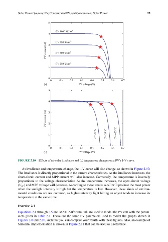
FIGURE 2.10 Effects of (a) solar irradiance and (b) temperature changes on a PV’s I–V curve.

As irradiance and temperature change, the I–V curve will also change, as shown in Figure 2.10.
The irradiance is directly proportional to the current characteristics. As the irradiance increases, the
short-circuit current and MPP current will also increase. Conversely, the temperature is inversely
proportional to the voltage characteristics. As the temperature increases, the open-circuit voltage
(V ) and MPP voltage will decrease. According to these trends, a cell will produce the most power
OC
when the sunlight intensity is high but the temperature is low. However, these kinds of environ-
mental conditions are not common, as higher-intensity light hitting an object tends to increase its
temperature at the same time.

Exercise 2.1
Equations 2.1 through 2.5 and MATLAB /Simulink are used to model the PV cell with the param-
®
eters given in Table 2.1. These are the same PV parameters used to model the graphs shown in
Figures 2.8 and 2.10, such that you can compare your results with these figures. Also, an example of
Simulink implementation is shown in Figure 2.11 that can be used as a reference.