Page 71 - Renewable Energy Devices and System with Simulations in MATLAB and ANSYS

58 Renewable Energy Devices and Systems with Simulations in MATLAB and ANSYS ®
®

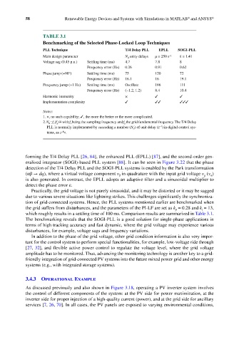
TABLE 3.1
Benchmarking of the Selected Phase-Locked Loop Techniques
PLL Technique T/4 Delay PLL EPLL SOGI-PLL
Main design parameter N d unity delays μ = 250 s −1 k = 1.41
Voltage sag (0.45 p.u.) Settling time (ms) 4.7 7.8 8
Frequency error (Hz) 0.26 0.91 0.62
Phase jump (+90°) Settling time (ms) 75 120 72
Frequency error (Hz) 16.1 16 19.1
Frequency jump (+1 Hz) Settling time (ms) Oscillate 186 111
Frequency error (Hz) (−1.2, 1.2) 8.4 10.4
Harmonic immunity × ✓ ✓
Implementation complexity ✓ ✓✓ ✓✓✓

Notes:
1. ×, no such capability; ✓, the more the better or the more complicated.

2.N d f s /f g /4 withf s being the sampling frequency andf g the grid fundamental frequency.The T/4 Delay

=
−1
PLL is normally implemented by cascading a number (N d ) of unit delay (z ) in digital control sys-
tems, as z –N d.
forming the T/4 Delay PLL [26, 84], the enhanced PLL (EPLL) [87], and the second-order gen-
eralized integrator (SOGI)-based PLL system [88]. It can be seen in Figure 3.22 that the phase
detection of the T/4 Delay PLL and the SOGI-PLL systems is enabled by the Park transformation
(αβ → dq), where a virtual voltage component v in quadrature with the input grid voltage v (v )
g
α
β
is also generated. In contrast, the EPLL adopts an adaptive filter and a sinusoidal multiplier to
detect the phase error ε.
Practically, the grid voltage is not purely sinusoidal, and it may be distorted or it may be sagged
due to various severe situations like lightning strikes. This challenges significantly the synchroniza-
tion of grid-connected systems. Hence, the PLL systems mentioned earlier are benchmarked when
the grid suffers from disturbances, and the parameters of the PI-LF are set as k = 0.28 and k = 13,
p
i
which roughly results in a settling time of 100 ms. Comparison results are summarized in Table 3.1.
The benchmarking reveals that the SOGI-PLL is a good solution for single-phase applications in
terms of high tracking accuracy and fast dynamic, where the grid voltage may experience various
disturbances, for example, voltage sags and frequency variations.
In addition to the phase of the grid voltage, other grid condition information is also very impor-
tant for the control system to perform special functionalities, for example, low-voltage ride through
[27, 32], and flexible active power control to regulate the voltage level, where the grid voltage
amplitude has to be monitored. Thus, advancing the monitoring technology is another key to a grid-
friendly integration of grid-connected PV systems into the future mixed power grid and other energy
systems (e.g., with integrated storage systems).

3.4.3 Operational Example
As discussed previously and also shown in Figure 3.18, operating a PV inverter system involves
the control of different components of the system: at the PV side for power maximization, at the
inverter side for proper injection of a high-quality current (power), and at the grid side for ancillary
services [7, 26, 70]. In all cases, the PV panels are exposed to varying environmental conditions,