Page 118 - Robot Builders Source Book - Gordon McComb

3.7 Drive with a Variable Moment of Inertia 107

Therefore, we show here some computation examples of Equation (3.178) made
with the MATHEMATICA program. For this purpose, let us decide about the values of
the parameters constituting this equation, as follows:
r 0 = 0.1m, r^O.lm/sec, r 0 = 5Nm, 7\ = IN sec.
In addition, we take three different values for the moving mass: m = 2kg, 3kg, and 4kg.
In keeping with these parameters and for each of the chosen mass values, we write
the needed expressions and obtain the solutions in graphic form as follows.
The calculations, as was mentioned above, were carried out for three different mass
values. This fact is reflected in the three curves on each graph shown in Figure 3.30a)
and b). The upper ones belong to the smallest mass value (in our case m = 2kg), and
the lowest curves to the largest mass (m = 4kg).
fl=w'[t]+w[t]*(.2+.5/(.l+.l*t))/(.l+.l*t)-2.5/(.l+.l*t)^2
yl=NDSolve[{fl==0,w[0]==0},w,{t,0,.l}]
zl=Plot[Evaluate[w[t] /.yl] ,{t,0,. 1}, AxesLabel-
>{"t,time","w,speed"}]
A
f2=w'[t]-hw[t]*(.2+.333/(.l+.l*t))/(.l+.l*t)-1.7/(.l+.l*t) 2
y2=NDSolve[{f2==0,w[0]==0},w,{t,0,.l}]
z2=Plot[Evaluate[w[t] /.y2] ,{t,0,. 1}, AxesLabel-
>{"t,time","w,speed"}]
A
f3=w'[t]+w[t]*(.2+.25/(.l+.l*t))/(.l+.l*t)-1.25/(.l+.l*t) 2
y3=NDSolve[{f3==0,w[0]==0},w,{t,0,.l}]
z3=Plot[Evaluate[w[t]/.y3],{t,0,.l},AxesLabel-
>{%time","w,speed"}]
xl=Show[zl,z2,z3]
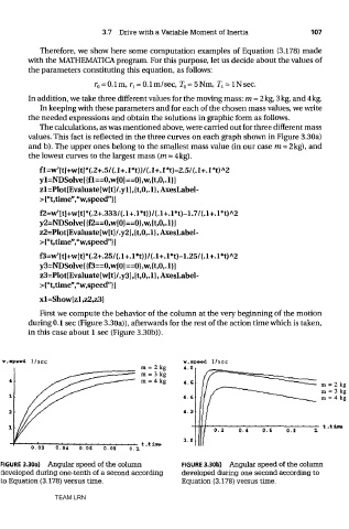
First we compute the behavior of the column at the very beginning of the motion
during 0.1 sec (Figure 3.30a)), afterwards for the rest of the action time which is taken,
in this case about 1 sec (Figure 3.30b)).

FIGURE 3.30a) Angular speed of the column FIGURE 3.30b) Angular speed of the column
developed during one-tenth of a second according developed during one second according to
to Equation (3.178) versus time. Equation (3.178) versus time.
TEAM LRN