Page 119 - Robot Builders Source Book - Gordon McComb

108 Dynamic Analysis of Drives

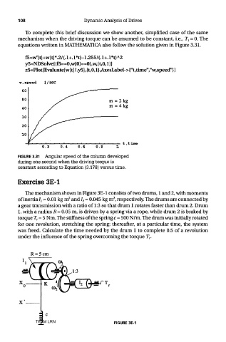
To complete this brief discussion we show another, simplified case of the same
mechanism when the driving torque can be assumed to be constant, i.e., 7\ = 0. The
equations written in MATHEMATICA also follow the solution given in Figure 3.31.

f5=w'[t]+w[t]*.2/(.l+.l*t)-1.255/(.l+.l*t)A2
y5=NDSolve[{f5==0,w[0] ==0},w,{t,0,1}]
z5=Plot[Evaluate[w[t]/.y5],{t,0,l} >AxesLabel->{"t,time","w,speed"}]

FIGURE 3.31 Angular speed of the column developed
during one second when the driving torque is
constant according to Equation (3.178) versus time.

Exercise 3E-1

The mechanism shown in Figure 3E-1 consists of two drums, 1 and 2, with moments
2
2
of inertia/! = 0.01 kg m and I 2 = 0.045 kg m , respectively. The drums are connected by
a gear transmission with a ratio of 1:3 so that drum 1 rotates faster than drum 2. Drum
1, with a radius R = 0.05 m, is driven by a spring via a rope, while drum 2 is braked by
torque T r = 5 Nm. The stiffness of the spring c - 500 N/m. The drum was initially rotated
for one revolution, stretching the spring; thereafter, at a particular time, the system
was freed. Calculate the time needed by the drum 1 to complete 0.5 of a revolution
under the influence of the spring overcoming the torque T r.

TEAM LRN FIGURE 3E-1