Page 161 - Robotics Designing the Mechanisms for Automated Machinery

4.4 Dynamic Accuracy 149

chosen from among a very wide range of possibilities, and Figure 4.13 shows a partial
graphical interpretation of a specific function with the displacement s, velocity s, and
acceleration s. While the graph shows the ideal shapes of these kinematic character-
istics, one can never actually achieve such curves, whatever the effort made to attain
accuracy in manufacturing. And the reason for this pessimistic note is the limited stiff-
ness of the links constituting the mechanism, with their deformation by external and
inertial forces. These deformations are usually too small to significantly alter the shape
of the displacement s(f). However, the first- and second-order derivatives, namely, the
velocity s and especially the acceleration s, can (and usually do) acquire significant
deflections or errors. Sometimes the errors in acceleration reach the order of magni-
tude of the nominal acceleration.
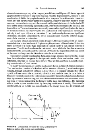
An example of such disturbed results (Figure 4.45) was obtained with an experi-
mental device in the Mechanical Engineering Department of Ben-Gurion University.
Here, a section of a cosine-type acceleration carried out by a cam-driven follower is
presented. The thicker line shows the calculated curve, while the thin line shows the
real data for the acceleration of the follower. Obviously, the higher the rotational speed
of the cam, the larger are the disturbances in the accelerations.
These errors should be estimated during the design process. It is worthwhile to see
how these disturbances appear in the dynamic model of the mechanism under con-
sideration. How can we foresee these errors? What are the analytical means of obtain-
ing an estimation of their values?
To clarify the discussion we use the mechanism shown in Figure 4.46 as an example.
This mechanism consists of a flywheel with a moment of inertia / 0, which drives gear
wheel z l through a shaft with stiffness q. Gear wheel z l is engaged with another wheel
z 2 which drives a cam (the eccentricity of which is e), and the latter, in turn, drives a
follower. The motion s(f) of the follower is described by the motion function and equals
11(0). By means of a connecting rod, the follower drives mass m and overcomes exter-
nal force E The rod connecting the follower to the mass has stiffness c 2. The damping
effects in the system are described by damping coefficients b l and b 2. These coeffi-
cients will help us to take into consideration the energy losses due to internal and

FIGURE 4.45 Comparison between the ideal and measured
follower motion of a cosine cam mechanism.