Page 176 - Satellite Communications, Fourth Edition

156 Chapter Six

direct and is the preferred method, with the guide operating in the
TE mode. The conical horn antenna may be used with linear or circu-
11
lar polarization, but in order to illustrate some of the important features,
linear polarization will be assumed.
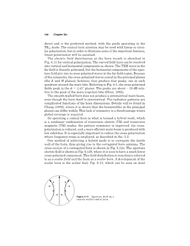
The electric field distribution at the horn mouth is sketched in
Fig. 6.11 for vertical polarization. The curved field lines can be resolved
into vertical and horizontal components as shown. The TEM wave in the
far field is linearly polarized, but the horizontal components of the aper-
ture field give rise to cross-polarized waves in the far-field region. Because
of the symmetry, the cross-polarized waves cancel in the principal planes
(the E and H planes); however, they produce four peaks, one in each
quadrant around the main lobe. Referring to Fig. 6.5, the cross-polarized
fields peak in the 45° planes. The peaks are about 19 dB rela-
tive to the peak of the main (copolar) lobe (Olver, 1992).
The smooth-walled horn does not produce a symmetrical main beam,
even though the horn itself is symmetrical. The radiation patterns are
complicated functions of the horn dimensions. Details will be found in
Chang (1989), where it is shown that the beamwidths in the principal
planes can differ widely. This lack of symmetry is a disadvantage where
global coverage is required.
By operating a conical horn in what is termed a hybrid mode, which
is a nonlinear combination of transverse electric (TE) and transverse
magnetic (TM) modes, the pattern symmetry is improved, the cross-
polarization is reduced, and a more efficient main beam is produced with
low sidelobes. It is especially important to reduce the cross-polarization
where frequency reuse is employed, as described in Sec. 5.2.
One method of achieving a hybrid mode is to corrugate the inside
wall of the horn, thus giving rise to the corrugated horn antenna. The
cross section of a corrugated horn is shown in Fig. 6.12a. The aperture
electric field is shown in Fig. 6.12b, where it is seen to have a much lower
cross-polarized component. This field distribution is sometimes referred
to as a scalar field and the horn as a scalar horn. A development of the
scalar horn is the scalar feed, Fig. 6.13, which can be seen on most

Figure 6.11 Aperture field in a
smooth-walled conical horn.