Page 216 - Schaum's Outline of Differential Equations

CHAP. 20] SOLVING SECOND-ORDER DIFFERENTIAL EQUATIONS 199

ZQ = 0. Then, using (20.3), we compute

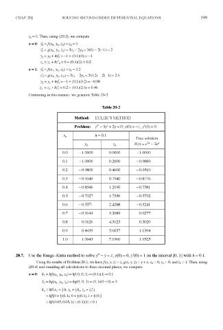
Continuing in this manner, we generate Table 20-2.

Table 20-2

Method: EULER' S METHOD
Problem: /' - 3/ + 2y = 0 ; y(0) = - 1 , /(O) = 0

ft = 0.1
x n
True solution
y n Zn Y(x) = e *-2<?
2
0.0 -1.0000 0.0000 -1.0000
0.1 -1.0000 0.2000 -0.9889
0.2 -0.9800 0.4600 -0.9510

0.3 -0.9340 0.7940 -0.8776

0.4 -0.8546 1.2190 -0.7581
0.5 -0.7327 1.7556 -0.5792
0.6 -0.5571 2.4288 -0.3241

0.7 -0.3143 3.2689 0.0277

0.8 0.0126 4.3125 0.5020
0.9 0.4439 5.6037 1.1304
1.0 1.0043 7.1960 1.9525

20.7. Use the Runge-Kutta method to solve y" -y = x; y(0) = 0, /(O) = 1 on the interval [0, 1] with h = 0.1.
Using the results of Problem 20.1, we have/(jc, y, z) = Z, g(x, y,z)=y + x,x Q = 0, y Q = 0, and z 0 = 1- Then, using
(20.4) and rounding all calculations to three decimal places, we compute: