Page 219 - Schaum's Outline of Differential Equations

202 SOLVING SECOND-ORDER DIFFERENTIAL EQUATIONS [CHAP. 20

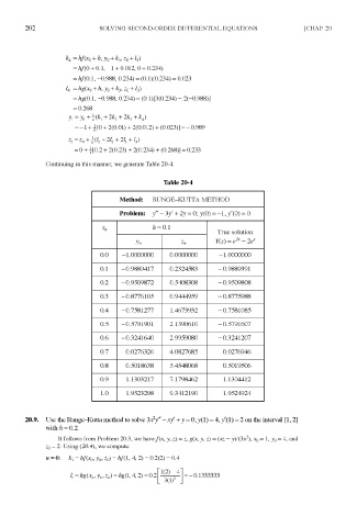
Continuing in this manner, we generate Table 20-4.

Table 20-4

Method: RUNGE-KUTTA METHOD
Problem: /' - 3/ + 2y = 0 ; y(0) = - 1 , /(O) = 0
h = 0.1
x n
True solution
y n z n Y(x) = e - 2e x
21
0.0 -1.0000000 0.0000000 -1.0000000
0.1 -0.9889417 0.2324583 -0.9889391

0.2 -0.9509872 0.5408308 -0.9509808
0.3 -0.8776105 0.9444959 -0.8775988

0.4 -0.7581277 1.4673932 -0.7581085
0.5 -0.5791901 2.1390610 -0.5791607
0.6 -0.3241640 2.9959080 -0.3241207

0.7 0.0276326 4.0827685 0.0276946

0.8 0.5018638 5.4548068 0.5019506
0.9 1.1303217 7.1798462 1.1304412

1.0 1.9523298 9.3412190 1.9524924

2
20.9. Use the Runge-Kutta method to solve 3.x /' -xy' + y = 0; y(l) = 4, /(I) = 2 on the interval [1,2]
with h = 0.2.
2
It follows from Problem 20.3, we have/(jc, y, z) = Z, g(x, y, z) = (xz — y)l(3x ), x 0 =l,y 0 = 4, and
ZQ = 2. Using (20.4), we compute: