Page 223 - Schaum's Outline of Theory and Problems of Advanced Calculus

214 MULTIPLE INTEGRALS [CHAP. 9

We can also consider the double integral as representing the mass of the region r assuming a
2
2
density varying as x þ y .
(c) Method 1: The double integral can be expressed as the iterated integral
2
x
x
ð 2 ð 2 ð 2 ( ð 2 ) ð 2 3 x
2 2 2 2 2 y
dx
ðx þ y Þ dy dx ¼ ðx þ y Þ dy dx ¼ x y þ
x¼1 y¼1 x¼1 y¼1 x¼1 3 y¼1
!
2 x 1 1006
ð 6
4 2
¼ x þ x dx ¼
x¼1 3 3 105
2
The integration with respect to y (keeping x constant) from y ¼ 1to y ¼ x corresponds formally
to summing in a vertical column (see Fig. 9-6). The subsequent integration with respect to x from x ¼ 1
to x ¼ 2corresponds to addition of contributions from all such vertical columns between x ¼ 1 and
x ¼ 2.
Method 2: The double integral can also be expressed as the iterated integral
( )
ð 4 ð 2 ð 4 ð 2 ð 4 3 2
2 2 2 2 x
ðx þ y Þ dx dy ¼ ðx þ y Þ dx dy ¼ þ xy 2 dy
p
p
y¼1 x¼ y ffiffi y¼1 x¼ y ffiffi y¼1 3 x¼ y ffiffi
p
!
8 2 y 5=2 1006
ð 4 3=2
y¼1 3 3 105
¼ þ 2y y dy ¼
In this case the vertical column of region r in Fig. 9-6 above is replaced by a horizontal column as
y to x ¼ 2
p ffiffiffi
in Fig. 9-7 above. Then the integration with respect to x (keeping y constant) from x ¼
corresponds to summing in this horizontal column. Subsequent integration with respect to y from
y ¼ 1to y ¼ 4corresponds to addition of contributions for all such horizontal columns between y ¼ 1
and y ¼ 4.
2
1 2
9.2. Find the volume of the region bound by the elliptic paraboloid z ¼ 4 x y and the plane
4
z ¼ 0.
Because of the symmetry of the elliptic paraboloid, the result can be obtained by multiplying the first
octant volume by 4.
2
2
Letting z ¼ 0yields 4x þ y ¼ 16. The limits of integration are determined from this equation. The
required volume is
p ffiffiffiffiffiffiffiffi
p ffiffiffiffiffiffiffiffi ! 2 4 x 2
2
ð ð 2 4 x 2 1 ð 2 1 y 3
2
2
4 4 x y 2 dy dx ¼ 4 4y x y dx
0 0 4 0 4 3
0
¼ 16
Hint: Use trigonometric substitutions to complete the integrations.
2 p ffiffiffiffiffiffiffiffiffiffiffiffiffi 2
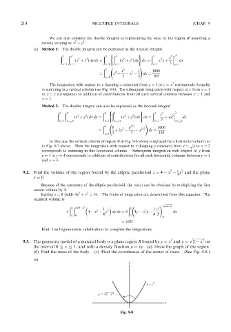
9.3. The geometric model of a material body is a plane region R bound by y ¼ x and y ¼ 2 x on
the interval 0 @ x @ 1, and with a density function ¼ xy (a) Draw the graph of the region.
(b) Find the mass of the body. (c) Find the coordinates of the center of mass. (See Fig. 9-8.)
(a)

Fig. 9-8