Page 228 - Schaum's Outline of Theory and Problems of Advanced Calculus

CHAP. 9] MULTIPLE INTEGRALS 219

We can also write the integration limits for r immediately on observing the region r, since for fixed ,
0
varies from ¼ 2to ¼ 3within the sector shown dashed in Fig. 9-13(a). An integration with respect to
from ¼ 0to ¼ 2 then gives the contribution from all sectors. Geometrically, d d represents the
area dA as shown in Fig. 9-13(a).

2 2
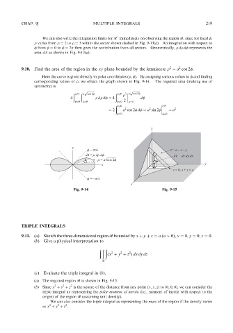
9.10. Find the area of the region in the xy plane bounded by the lemniscate ¼ a cos 2 .
Here the curve is given directly in polar coordinates ð ; Þ.By assigning various values to and finding
corresponding values of ,we obtain the graph shown in Fig. 9-14. The required area (making use of
symmetry) is
ffiffiffiffiffiffiffiffiffi
p ffiffiffiffiffiffiffiffiffi p
=4 a =4
ð ð cos 2 ð 3 a cos 2

4 d d ¼ 4 d
¼0 ¼0 ¼0 2 ¼0
ð =4 =4
2
2
¼ 2 a cos 2 d ¼ a sin 2 ¼ a 2

¼0 ¼0

Fig. 9-14 Fig. 9-15

TRIPLE INTEGRALS

9.11. (a) Sketch the three-dimensional region r bounded by x þ y þ z ¼ a ða > 0Þ; x ¼ 0; y ¼ 0; z ¼ 0.
(b) Give a physical interpretation to

ððð
2
2
2
ðx þ y þ z Þ dx dy dz
r
(c) Evaluate the triple integral in (b).
(a) The required region r is shown in Fig. 9-15.
2
2
2
(b)Since x þ y þ z is the square of the distance from any point ðx; y; zÞ to ð0; 0; 0Þ,we can consider the
triple integral as representing the polar moment of inertia (i.e., moment of inertia with respect to the
origin) of the region r (assuming unit density).
We can also consider the triple integral as representing the mass of the region if the density varies
2
2
2
as x þ y þ z .