Page 49 - Schaum's Outline of Theory and Problems of Advanced Calculus

40 FUNCTIONS, LIMITS, AND CONTINUITY [CHAP. 3

2
EXAMPLES. 1. If to each number in 1 @ x @ 1weassociate a number y given by x ,thenthe interval
2
1 @ x @ 1isthe domain. The rule y ¼ x generates the range 1 @ y @ 1. The totality
is a function f .
2
1 2
1
1
The functional image of x is given by y ¼ f ðxÞ¼ x . For example, f ð Þ¼ ð Þ ¼ is the
9
3
3
1
image of with respect to the function f .
3
2. The sequences of Chapter 2 may be interpreted as functions. For infinite sequences consider the
domain as the set of positive integers. The rule is the definition of u n , and the range is generated
1
by this rule. To illustrate, let u n ¼ with n ¼ 1; 2; ... . Then the range contains the elements
n
1 1 1
1
1; ; ; ; .. . . Ifthe function is denoted by f ,then we may write f ðnÞ¼ .
2 3 4 n
As you read this chapter, reviewing Chapter 2 will be very useful, and in particular com-
paring the corresponding sections.
3. With each time t after the year 1800 we can associate a value P for the population of the United
States. The correspondence between P and t defines a function, say F, and we can write
P ¼ FðtÞ.
4. For the present, both the domain and the range of a function have been restricted to sets of real
numbers. Eventually this limitation will be removed. To get the flavor for greater generality,
think of a map of the world on a globe with circles of latitude and longitude as coordinate
curves. Assume there is a rule that corresponds this domain to a range that is a region of a
plane endowed with a rectangular Cartesian coordinate system. (Thus, a flat map usable for
navigation and other purposes is created.) The points of the domain are expressed as pairs of
numbers ð ; Þ and those of the range by pairs ðx; yÞ. These sets and a rule of correspondence
constitute a function whose independent and dependent variables are not single real numbers;
rather, they are pairs of real numbers.
GRAPH OF A FUNCTION
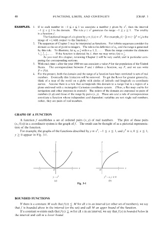
A function f establishes a set of ordered pairs ðx; yÞ of real numbers. The plot of these pairs
ðx; f ðxÞÞ in a coordinate system is the graph of f . The result can be thought of as a pictorial representa-
tion of the function.
2 2
For example, the graphs of the functions described by y ¼ x , 1 @ x @ 1, and y ¼ x,0 @ x @ 1,
y A 0 appear in Fig. 3-1.

Fig. 3-1

BOUNDED FUNCTIONS

If there is a constant M such that f ðxÞ @ M for all x in an interval (or other set of numbers), we say
that f is bounded above in the interval (or the set) and call M an upper bound of the function.
If a constant m exists such that f ðxÞ A m for all x in an interval, we say that f ðxÞ is bounded below in
the interval and call m a lower bound.