Page 175 - Schaum's Outline of Theory and Problems of Electric Circuits

HIGHER-ORDER CIRCUITS AND COMPLEX FREQUENCY
164

Fig. 8-5 [CHAP. 8

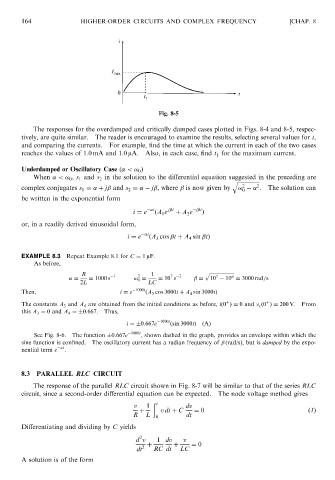
The responses for the overdamped and critically damped cases plotted in Figs. 8-4 and 8-5, respec-
tively, are quite similar. The reader is encouraged to examine the results, selecting several values for t,
and comparing the currents. For example, find the time at which the current in each of the two cases
reaches the values of 1.0 mA and 1.0 mA. Also, in each case, find t for the maximum current.
1
Underdamped or Oscillatory Case ð <! 0 Þ
When <! 0 , s 1 and s 2 in the solution to the differential equation suggested in the preceding are
q ffiffiffiffiffiffiffiffiffiffiffiffiffiffiffiffi
2
2
complex conjugates s 1 ¼ þ j and s 2 ¼ j , where is now given by ! . The solution can
0
be written in the exponential form
i ¼ e t ðA 1 e j t þ A 2 e j t Þ
or, in a readily derived sinusoidal form,
i ¼ e t ðA 3 cos t þ A 4 sin tÞ

EXAMPLE 8.3 Repeat Example 8.1 for C ¼ 1 mF.
As before,
p ffiffiffiffiffiffiffiffiffiffiffiffiffiffiffiffiffiffiffiffi
R 1
7 2
2
6
7
¼ ¼ 1000 s 1 ! 0 ¼ ¼ 10 s ¼ 10 10 ¼ 3000 rad=s
2L LC
Then, i ¼ e 1000t ðA 3 cos 3000t þ A 4 sin 3000tÞ
þ
þ
The constants A 3 and A 4 are obtained from the initial conditions as before, ið0 Þ¼ 0 and v c ð0 Þ¼ 200 V. From
this A 3 ¼ 0 and A 4 ¼ 0:667. Thus,
i ¼ 0:667e 1000t ðsin 3000tÞðAÞ
See Fig. 8-6. The function 0:667e 1000t , shown dashed in the graph, provides an envelope within which the
sine function is confined. The oscillatory current has a radian frequency of (rad/s), but is damped by the expo-
nential term e t .

8.3 PARALLEL RLC CIRCUIT
The response of the parallel RLC circuit shown in Fig. 8-7 will be similar to that of the series RLC
circuit, since a second-order differential equation can be expected. The node voltage method gives
ð
v 1 t dv
þ vdt þ C ¼ 0 ð1Þ
R L 0 dt
Differentiating and dividing by C yields
2
d v 1 dv v
þ þ ¼ 0
2
dt RC dt LC
A solution is of the form