Page 179 - Schaum's Outline of Theory and Problems of Electric Circuits

HIGHER-ORDER CIRCUITS AND COMPLEX FREQUENCY
168
2 [CHAP. 8
d i 1 R 1 L 1 þ R 2 L 1 þ R 1 L 2 di 1 R 1 R 2 R 2 V
þ þ i 1 ¼ ð7Þ
2
dt L 1 L 2 dt L 1 L 2 L 1 L 2
The steady-state solution of (7) is evidently i ð1Þ ¼ V=R ; the transient solution will be determined
1
1
by the roots s 1 and s 2 of
2 R 1 L 1 þ R 2 L 1 þ R 1 L 2 R 1 R 2
s þ s þ ¼ 0
L 1 L 2 L 1 L 2
together with the initial conditions

V
di 1
þ
i 1 ð0 Þ¼ 0 ¼
dt 0 þ L 1
(both i 1 and i 2 must be continuous at t ¼ 0). Once the expression for i 1 is known, that for i 2 follows
from (4).
There will be a damping factor that insures the transient will ultimately die out. Also, depending
on the values of the four circuit constants, the transient can be overdamped or underdamped, which is
oscillatory. In general, the current expression will be
V
i 1 ¼ðtransientÞþ
R 1
The transient part will have a value of V=R 1 at t ¼ 0 and a value of zero as t !1.

8.5 COMPLEX FREQUENCY
We have examined circuits where the driving function was a constant (e.g., V ¼ 50:0 V), a sinusoidal
function (e.g., v ¼ 100:0 sin ð500t þ 308Þ (V), or an exponential function, e.g., v ¼ 10e 5t (V). In this
section, we introduce a complex frequency, s, which unifies the three functions and will simplify the
analysis, whether the transient or steady-state response is required.
We begin by expressing the exponential function in the equivalent cosine and sine form:

e jð!tþ Þ ¼ cos ð!t þ Þþ j sin ð!t þ Þ
We will focus exclusively on the cosine term cos ð!t þ Þ¼ Re e jð!tþ Þ and for convenience drop the
t
prefix Re. Introducing a constant A and the factor e ,
t
t jð!tþ Þ
j st
j ð þj!Þt
Ae e ) Ae cos ð!t þ Þ Ae e ¼ Ae e where s ¼ þ j!
1
The complex frequency s ¼ þ j! has units s , and !, as we know, has units rad/s. Consequently,
1
the units on must also be s . This is the neper frequency with units Np/s. If both and ! are

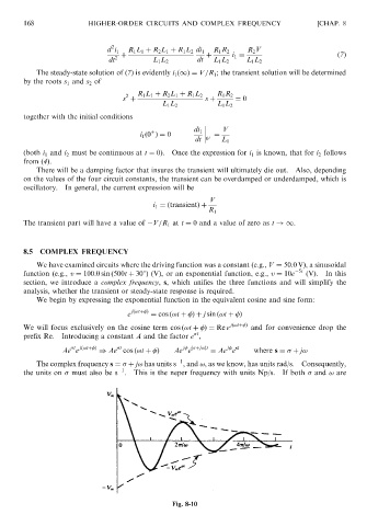
Fig. 8-10