Page 95 - Schaum's Outline of Theory and Problems of Electric Circuits

84
Therefore, AMPLIFIERS AND OPERATIONAL AMPLIFIER CIRCUITS [CHAP. 5
v o:c: ¼ 5ð19:8Þ¼ 99 V v Th ¼ v o:c: ¼ 99 V
i s:c: ¼ 99=3 ¼ 33 A R Th ¼ v o:c: =i s:c: ¼ 3
The The ´ venin equivalent is shown in Fig. 5-32.
(b) With the load R l connected, we have
2
R l 99R l v 2
v 2 ¼ v Th ¼ and p ¼
R l þ R Th R l þ 3 R l
Table 5-3 shows the voltage across the load and the power dissipated in it for the given seven values of
R l . The load voltage is at its maximum when R l ¼1. However, power delivered to R l ¼1 is zero.
Power delivered to R l is maximum at R l ¼ 3
, which is equal to the output resistance of the amplifier.
Table 5-3

R l ;
v 2 ; V p; W
0.5 14.14 400.04
1 24.75 612.56
3 49.50 816.75
5 61.88 765.70
10 76.15 579.94
100 96.12 92.38
1000 98.70 9.74

þ
5.2 In the circuits of Figs. 5-4 and 5-5 let R 1 ¼ 1k
and R 2 ¼ 5k
. Find the gains G ¼ v 2 =v s in

Fig. 5-4 and G ¼ v 2 =v s in Fig. 5-5 for k ¼ 1, 2, 4, 6, 8, 10, 100, 1000, and 1. Compare the
results.
From (5) in Example 5.3, at R 1 ¼ 1k
and R 2 ¼ 5k
we have
5k
v 2
þ
G ¼ ¼ ð31Þ
v s 6 k
In Example 5.4 we found
5k
v 2

G ¼ ¼ ð32Þ
v s 6 þ k

þ
þ
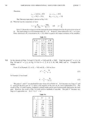
The gains G and G are calculated for nine values of k in Table 5-4. As k becomes very large, G and

G approach the limit gain of 5, which is the negative of the ratio R 2 =R 1 and is independent of k. The
circuit of Fig. 5-5 (with negative feedback) is always stable and its gain monotonically approaches the limit
þ
gain. However, the circuit of Fig. 5-4 (with positive feedback) is unstable. The gain G becomes very
þ
large as k approaches six. At k ¼ 6, G ¼1.
Table 5-4
k G þ G
1 1:0 0:71
2 2:5 1:25
4 10:0 2:00
6 1 2:50
8 20:0 2:86
10 12:5 3:12
100 5:32 4:72
1000 5:03 4:97
1 5:00 5:00