Page 91 - Schaum's Outline of Theory and Problems of Electric Circuits

AMPLIFIERS AND OPERATIONAL AMPLIFIER CIRCUITS
80

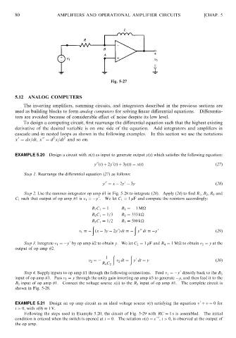
Fig. 5-27 [CHAP. 5

5.12 ANALOG COMPUTERS
The inverting amplifiers, summing circuits, and integrators described in the previous sections are
used as building blocks to form analog computers for solving linear differential equations. Differentia-
tors are avoided because of considerable effect of noise despite its low level.
To design a computing circuit, first rearrange the differential equation such that the highest existing
derivative of the desired variable is on one side of the equation. Add integrators and amplifiers in
cascade and in nested loops as shown in the following examples. In this section we use the notations
0
2
2
00
x ¼ dx=dt, x ¼ d x=dt and so on.
EXAMPLE 5.20 Design a circuit with xðtÞ as input to generate output yðtÞ which satisfies the following equation:
00
0
y ðtÞþ 2y ðtÞþ 3yðtÞ¼ xðtÞ ð27Þ
Step 1. Rearrange the differential equation (27) as follows:

0
00
y ¼ x 2y 3y ð28Þ
Step 2. Use the summer-integrator op amp #1 in Fig. 5-28 to integrate (28). Apply (24) to find R 1 ; R 2 ; R 3 and
C 1 such that output of op amp #1 is v 1 ¼ y . 0 We let C 1 ¼ 1 mF and compute the resistors accordingly:
R 1 C 1 ¼ 1 R 1 ¼ 1M
R 2 C 1 ¼ 1=3 R 2 ¼ 333 k
R 3 C 1 ¼ 1=2 R 3 ¼ 500 k
ð ð
0
00
v 1 ¼ ðx 3y 2y Þ dt ¼ y dt ¼ y 0 ð29Þ
0
Step 3. Integrate v 1 ¼ y by op amp #2 to obtain y. We let C 2 ¼ 1 mF and R 4 ¼ 1M
to obtain v 2 ¼ y at the
output of op amp #2.
ð ð
1
0
v 2 ¼ v 2 dt ¼ y dt ¼ y ð30Þ
R 4 C 2
0
Step 4. Supply inputs to op amp #1 through the following connections. Feed v 1 ¼ y directly back to the R 3
input of op amp #1. Pass v 2 ¼ y through the unity gain inverting op amp #3 to generate y, and then feed it to the
R 2 input of op amp #1. Connect the voltage source xðtÞ to the R 1 input of op amp #1. The complete circuit is
shown in Fig. 5-28.

0
EXAMPLE 5.21 Design an op amp circuit as an ideal voltage source vðtÞ satisfying the equation v þ v ¼ 0 for
t > 0, with vð0Þ¼ 1V.
Following the steps used in Example 5.20, the circuit of Fig. 5-29 with RC ¼ 1 s is assembled. The initial
t
condition is entered when the switch is opened at t ¼ 0. The solution vðtÞ¼ e , t > 0, is observed at the output of
the op amp.