Page 259 - Sensing, Intelligence, Motion : How Robots and Humans Move in an Unstructured World

234 MOTION PLANNING FOR TWO-DIMENSIONAL ARM MANIPULATORS

5.6 REVOLUTE–PRISMATIC (RP) ARM WITH PERPENDICULAR
LINKS

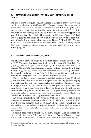
The arm is shown in Figure 5.1d. An example of the arm’s interaction with two
circular obstacles is shown in Figure 5.25a. C-space images of the corresponding
virtual obstacles and of the M-line are shown in Figure 5.25b. The path gener-
ated under the motion planning algorithm passes through points S, 1, 2,..., 9,T .
Although the arm’s configuration and its interaction with obstacles appear to be
quite different from those of the RP arm with parallel links (Figure 5.1c), both
arm manipulators turn out to be very similar from the standpoint of path plan-
ning. Visually this is evident when comparing Figures 5.24 and 5.25: Whereas
the W-space looks quite different for both arms, their C-spaces look very similar.
The reader is therefore referred to the previous section for analysis and motion
planning algorithm.

5.7 PRISMATIC–REVOLUTE (PR) ARM

The PR arm is shown in Figure 5.1e. A more detailed sketch appears in Fig-
ure 5.26. The arm’s first joint value is the variable length of its first link, 0 ≤
l 1 ≤ l 1max . The second joint value is angle θ 2 . The length of second link, l 2 ,is
constant. The arm’s W-space boundary is a combination of a rectangle with sides
of length l 1max and 2l 2 , respectively, and two semicircles of radius l 2 attached to
the rectangle, as shown in Figure 5.26. As before, assume that no obstacles may
interfere with the part of link l 1 as it moves outside of W-space. 6
The two circles of radius l 2 centered at the limit positions O and O 1 of link
l 1 are called the limit areas of arm’s W-space. Note that any point belonging
to a limit area has only one corresponding arm solution, whereas any point
of W-space that is outside the limit areas has two possible arm solutions. For
example, in Figure 5.26 a single arm solution exists for point P ,and twoarm
solutions exist for point P 1 . As we will see, for the path planning purposes this
peculiarity makes the arm distinct from those considered so far and leads to a
combination of features of the algorithms for those arms.
An obstacle is considered to be inside the limit area if only one arm solution
exists for all points of the obstacle virtual line. An obstacle is outside the limit
area if two arm solutions exist for all points of the obstacle virtual line. An
intermediate situation, referred to as partially inside the limit area, is when some
points of the obstacle virtual line have one solution and some other points have
two solutions.
Consider three circular obstacles A, B, and C (Figure 5.27a), positioned out-
side, partially inside, and fully inside the limit areas of the arm W-space, respec-
tively. Positions of the link endpoints at some points of the corresponding virtual

6 Incorporating that part of the arm body into the algorithm is very easy because link l 1 moves always
along the same line.