Page 162 - Separation process engineering

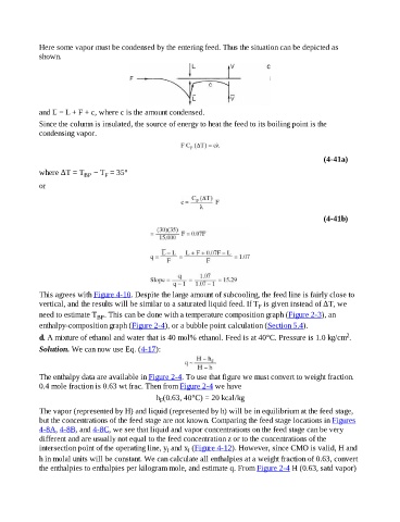
Here some vapor must be condensed by the entering feed. Thus the situation can be depicted as
shown.

and = L + F + c, where c is the amount condensed.

Since the column is insulated, the source of energy to heat the feed to its boiling point is the
condensing vapor.

(4-41a)

where ΔT = T − T = 35°
F
BP
or

(4-41b)

This agrees with Figure 4-10. Despite the large amount of subcooling, the feed line is fairly close to
vertical, and the results will be similar to a saturated liquid feed. If T is given instead of ΔT, we
F
need to estimate T . This can be done with a temperature composition graph (Figure 2-3), an
BP
enthalpy-composition graph (Figure 2-4), or a bubble point calculation (Section 5.4).

2
d. A mixture of ethanol and water that is 40 mol% ethanol. Feed is at 40°C. Pressure is 1.0 kg/cm .
Solution. We can now use Eq. (4-17):

The enthalpy data are available in Figure 2-4. To use that figure we must convert to weight fraction.
0.4 mole fraction is 0.63 wt frac. Then from Figure 2-4 we have
h (0.63, 40°C) = 20 kcal/kg
F

The vapor (represented by H) and liquid (represented by h) will be in equilibrium at the feed stage,
but the concentrations of the feed stage are not known. Comparing the feed stage locations in Figures
4-8A, 4-8B, and 4-8C, we see that liquid and vapor concentrations on the feed stage can be very
different and are usually not equal to the feed concentration z or to the concentrations of the
intersection point of the operating line, y and x (Figure 4-12). However, since CMO is valid, H and
I
I
h in molal units will be constant. We can calculate all enthalpies at a weight fraction of 0.63, convert
the enthalpies to enthalpies per kilogram mole, and estimate q. From Figure 2-4 H (0.63, satd vapor)