Page 256 - Separation process engineering

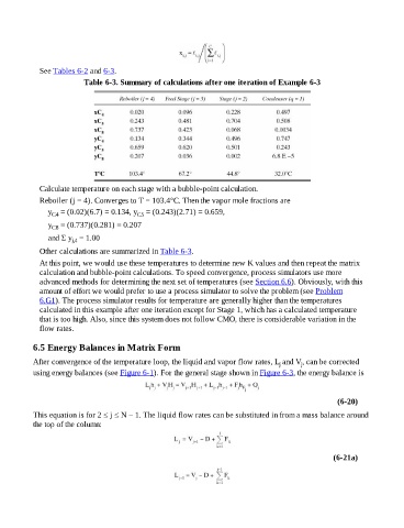
See Tables 6-2 and 6-3.

Table 6-3. Summary of calculations after one iteration of Example 6-3

Calculate temperature on each stage with a bubble-point calculation.

Reboiler (j = 4). Converges to T = 103.4°C. Then the vapor mole fractions are
y = (0.02)(6.7) = 0.134, y = (0.243)(2.71) = 0.659,
C5
C4
y = (0.737)(0.281) = 0.207
C8
and Σ y = 1.00
i,4
Other calculations are summarized in Table 6-3.

At this point, we would use these temperatures to determine new K values and then repeat the matrix
calculation and bubble-point calculations. To speed convergence, process simulators use more
advanced methods for determining the next set of temperatures (see Section 6.6). Obviously, with this
amount of effort we would prefer to use a process simulator to solve the problem (see Problem
6.G1). The process simulator results for temperature are generally higher than the temperatures
calculated in this example after one iteration except for Stage 1, which has a calculated temperature
that is too high. Also, since this system does not follow CMO, there is considerable variation in the
flow rates.

6.5 Energy Balances in Matrix Form

After convergence of the temperature loop, the liquid and vapor flow rates, L and V, can be corrected
j
j
using energy balances (see Figure 6-1). For the general stage shown in Figure 6-3, the energy balance is

(6-20)

This equation is for 2 ≤ j ≤ N − 1. The liquid flow rates can be substituted in from a mass balance around
the top of the column:

(6-21a)