Page 182 - Shigley's Mechanical Engineering Design

bud29281_ch04_147-211.qxd 11/27/09 2:55PM Page 157 ntt 203:MHDQ196:bud29281:0073529281:bud29281_pagefiles:

Deflection and Stiffness 157

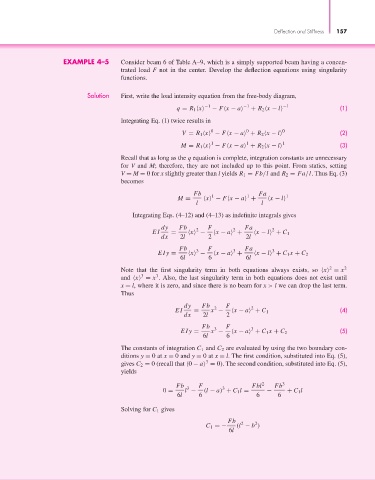
EXAMPLE 4–5 Consider beam 6 of Table A–9, which is a simply supported beam having a concen-
trated load F not in the center. Develop the deflection equations using singularity
functions.

Solution First, write the load intensity equation from the free-body diagram,
−1 −1 −1
q = R 1 x − F x − a + R 2 x − l (1)
Integrating Eq. (1) twice results in
0 0 0
V = R 1 x − F x − a + R 2 x − l (2)
1 1 1
M = R 1 x − F x − a + R 2 x − l (3)
Recall that as long as the q equation is complete, integration constants are unnecessary
for V and M; therefore, they are not included up to this point. From statics, setting
V = M = 0 for x slightly greater than l yields R 1 = Fb/l and R 2 = Fa/l. Thus Eq. (3)
becomes

Fb 1 1 Fa 1
M = x − F x − a + x − l
l l
Integrating Eqs. (4–12) and (4–13) as indefinite integrals gives
dy Fb 2 F 2 Fa 2
EI = x − x − a + x − l + C 1
dx 2l 2 2l
Fb 3 F 3 Fa 3
EIy = x − x − a + x − l + C 1 x + C 2
6l 6 6l
2
Note that the first singularity term in both equations always exists, so x = x 2
3
3
and x = x . Also, the last singularity term in both equations does not exist until
x = l, where it is zero, and since there is no beam for x > l we can drop the last term.
Thus
dy Fb 2 F 2
EI = x − x − a + C 1 (4)
dx 2l 2
Fb 3 F 3
EIy = x − x − a + C 1 x + C 2 (5)
6l 6
The constants of integration C 1 and C 2 are evaluated by using the two boundary con-
ditions y = 0 at x = 0 and y = 0 at x = l. The first condition, substituted into Eq. (5),
3
gives C 2 = 0 (recall that 0 − a = 0). The second condition, substituted into Eq. (5),
yields

Fb 3 F 3 Fbl 2 Fb 3
0 = l − (l − a) + C 1 l = − + C 1 l
6l 6 6 6
Solving for C 1 gives
Fb 2 2
C 1 =− (l − b )
6l