Page 274 - Shigley's Mechanical Engineering Design

bud29281_ch05_212-264.qxd 11/27/2009 6:46 pm Page 249 pinnacle s-171:Desktop Folder:Temp Work:Don't Delete (Jobs):MHDQ196/Budynas:

Failures Resulting from Static Loading 249
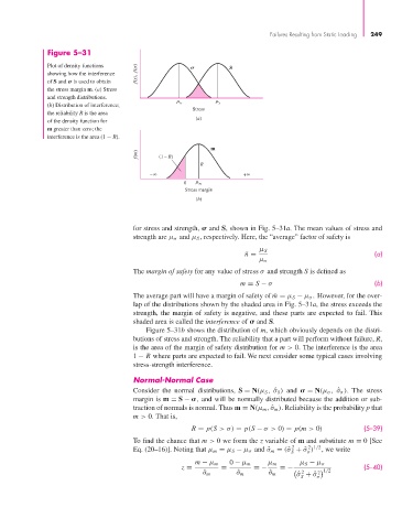
Figure 5–31

Plot of density functions S
showing how the interference f(s), f( )
of S and is used to obtain
the stress margin m. (a) Stress
and strength distributions.

(b) Distribution of interference; s
Stress
the reliability R is the area
(a)
of the density function for
m greater than zero; the
interference is the area (1 − R).
m
f(m) (1 – R)
R
– +
0 m
Stress margin
(b)

for stress and strength, and S, shown in Fig. 5–31a. The mean values of stress and
strength are μ σ and μ S , respectively. Here, the “average” factor of safety is
μ S
¯ n = (a)
μ σ
The margin of safety for any value of stress σ and strength S is defined as
m = S − σ (b)
The average part will have a margin of safety of ¯m = μ S − μ σ . However, for the over-
lap of the distributions shown by the shaded area in Fig. 5–31a, the stress exceeds the
strength, the margin of safety is negative, and these parts are expected to fail. This
shaded area is called the interference of and S.
Figure 5–31b shows the distribution of m, which obviously depends on the distri-
butions of stress and strength. The reliability that a part will perform without failure, R,
is the area of the margin of safety distribution for m > 0. The interference is the area
1 − R where parts are expected to fail. We next consider some typical cases involving
stress-strength interference.

Normal-Normal Case
Consider the normal distributions, S = N(μ S , ˆσ S ) and = N(μ σ , ˆσ σ ). The stress
margin is m = S − , and will be normally distributed because the addition or sub-
traction of normals is normal. Thus m = N(μ m , ˆσ m ). Reliability is the probability p that
m > 0. That is,
R = p(S >σ) = p(S − σ> 0) = p(m > 0) (5–39)
To find the chance that m > 0 we form the z variable of m and substitute m = 0 [See
2
2 1/2
Eq. (20–16)]. Noting that μ m = μ S − μ σ and ˆσ m = (ˆσ +ˆσ ) , we write
S σ
m − μ m 0 − μ m μ m μ S − μ σ
z = = =− =− 1/2 (5–40)
ˆ σ +ˆσ
ˆ σ m ˆ σ m ˆ σ m 2 2
S σ