Page 279 - Shigley's Mechanical Engineering Design

bud29281_ch05_212-264.qxd 11/27/2009 6:46 pm Page 254 pinnacle s-171:Desktop Folder:Temp Work:Don't Delete (Jobs):MHDQ196/Budynas:

254 Mechanical Engineering Design

1 1

R R 2
2

R 1 1 R 1 1
(a) (b)
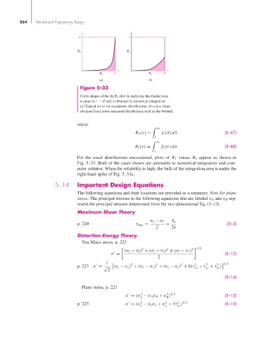
Figure 5–33

Curve shapes of the R 1 R 2 plot. In each case the shaded area
is equal to 1 − R and is obtained by numerical integration.
(a) Typical curve for asymptotic distributions; (b) curve shape
obtained from lower truncated distributions such as the Weibull.

where
∞

R 1 (x) = f 1 (S) dS (5–47)
x

∞
R 2 (x) = f 2 (σ) dσ (5–48)
x
For the usual distributions encountered, plots of R 1 versus R 2 appear as shown in
Fig. 5–33. Both of the cases shown are amenable to numerical integration and com-
puter solution. When the reliability is high, the bulk of the integration area is under the
right-hand spike of Fig. 5–33a.
5–14 Important Design Equations

The following equations and their locations are provided as a summary. Note for plane
stress: The principal stresses in the following equations that are labeled σ A and σ B rep-
resent the principal stresses determined from the two-dimensional Eq. (3–13).
Maximum Shear Theory

σ 1 − σ 3 S y
p. 220 τ max = = (5–3)
2 2n
Distortion-Energy Theory
Von Mises stress, p. 223

2 2 2 1/2
(σ 1 − σ 2 ) + (σ 2 − σ 3 ) + (σ 3 − σ 1 )
(5–12)
σ =
2
1/2
1 2 2 2 2 2 2

p. 223 σ = √ (σ x − σ y ) + (σ y − σ z ) + (σ z − σ x ) + 6(τ xy + τ + τ )
yz
zx
2
(5–14)
Plane stress, p. 223
2 1/2
2

σ = (σ − σ A σ B + σ ) (5–13)
A B
2
2
2
p. 223 σ = (σ − σ x σ y + σ + 3τ ) 1/2 (5–15)

x y xy