Page 277 - Six Sigma Demystified

Part 3 s i x s i g m a to o l s 257

licating the experiment, and then implement control mechanisms on the
significant factors as part of the improve stage.

• To model the process for prediction, run a central composite design (de-
scribed in the Glossary and applied as discussed in the “Response Surface
Analysis” topic below). It’s possible the screening design can be extended
with just a few experimental conditions to satisfy this requirement.
• To optimize the process by relocating it to a region of maximum yield,
proceed to response surface analysis (discussed below) or evolutionary
operation techniques (discussed earlier).

Factorial Designs

Minitab

Enter the experimental results in a column (one result for each run), and then
use Stat\DOE\Factorial\Analyze Factorial Design to select the column contain-
ing the response data. Use the “Terms” button to specify only first-order terms
for the initial screening analysis.
(For designs not created in Minitab, select the “Factors” button, and then select
the “Low/High” and “Designs” buttons to define factor levels and select a design
and optional center points, as described earlier.)
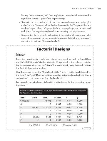
For example, the initial analysis (partial results shown) for the preceding exper-
iment are

Factorial Fit: Response versus a, B, C, D, E, and F—Estimated Effects and Coefficients
for Response (Coded units)

Term Effect Coef. SE Coef. T p
Constant –88,038 14,337 –6.14 0.000
A 1 0 14,337 0.00 1.000
B –24,432 –12,216 14,337 –0.85 0.416
C 3 2 14,337 0.00 1.000
D –1 0 14,337 0.00 1.000
E 21,362 10,681 14,337 0.75 0.475
F –1 0 14,337 0.00 1.000

2
S = 57347.0 R = 12.46% R (adj) = 0.00%
2
(Continued)