Page 415 - Six Sigma Demystified

Part 3 S i x S i g m a To o l S 395

the log of the standard deviation (of the replicated trials) indicates a slope of
1.462 in Figure F.53. Since this is close to 1.5, a reciprocal square root transfor-
mation will be applied so that the transformed y = 1/ y .
t
Box and Cox (1964) developed an iterative approach for determining an
optimal λ that minimizes the sum of squares error term. Myers and Montgom-
ery (1995) provide an example of this approach. A sample Minitab output
using the preceding example’s data is shown in Figure F.54.
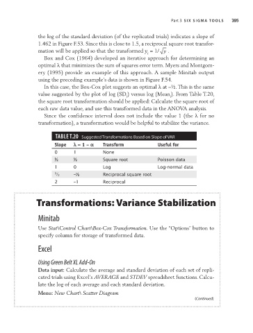
In this case, the Box-Cox plot suggests an optimal λ at –½. This is the same
value suggested by the plot of log (SD ) versus log (Mean ). From Table T.20,
i
i
the square root transformation should be applied: Calculate the square root of
each raw data value, and use this transformed data in the ANOVA analysis.
Since the confidence interval does not include the value 1 (the λ for no
transformation), a transformation would be helpful to stabilize the variance.

TAbLe T.20 Suggested Transformations Based on Slope of VaR
Slope  = 1 – a Transform Useful for
0 1 None
½ ½ Square root Poisson data
1 0 Log Log-normal data
3 / 2 –½ Reciprocal square root
2 –1 Reciprocal

Transformations: Variance Stabilization

Minitab

Use Stat\Control Chart\Box-Cox Transformation. Use the “Options” button to
specify column for storage of transformed data.
Excel

Using Green Belt XL Add-On
Data input: Calculate the average and standard deviation of each set of repli-
cated trials using Excel’s AVERAGE and STDEV spreadsheet functions. Calcu-
late the log of each average and each standard deviation.
Menu: New Chart\ Scatter Diagram
(Continued)