Page 73 - Six Sigma for electronics design and manufacturing

Six Sigma for Electronics Design and Manufacturing
42

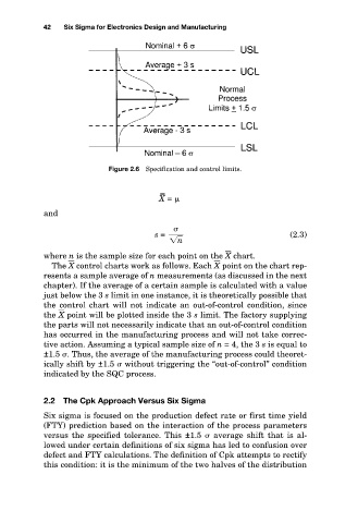
Figure 2.6 Specification and control limits.

– –
X =
and

s = (2.3)
n
where n is the sample size for each point on the X chart.
The X control charts work as follows. Each X point on the chart rep-
resents a sample average of n measurements (as discussed in the next
chapter). If the average of a certain sample is calculated with a value
just below the 3 s limit in one instance, it is theoretically possible that
the control chart will not indicate an out-of-control condition, since
the X point will be plotted inside the 3 s limit. The factory supplying
the parts will not necessarily indicate that an out-of-control condition
has occurred in the manufacturing process and will not take correc-
tive action. Assuming a typical sample size of n = 4, the 3 s is equal to
±1.5 . Thus, the average of the manufacturing process could theoret-
ically shift by ±1.5 without triggering the “out-of-control” condition
indicated by the SQC process.

2.2 The Cpk Approach Versus Six Sigma
Six sigma is focused on the production defect rate or first time yield
(FTY) prediction based on the interaction of the process parameters
versus the specified tolerance. This ±1.5 average shift that is al-
lowed under certain definitions of six sigma has led to confusion over
defect and FTY calculations. The definition of Cpk attempts to rectify
this condition: it is the minimum of the two halves of the distribution