Page 72 - Six Sigma for electronics design and manufacturing

The Elements of Six Sigma and Their Determination
41
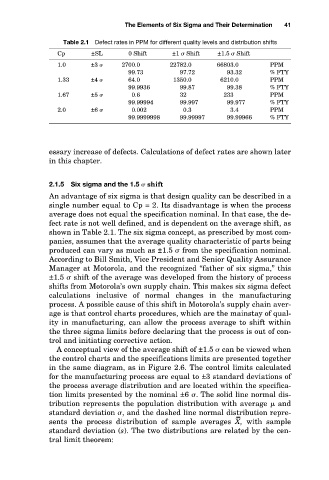
Table 2.1 Defect rates in PPM for different quality levels and distribution shifts
±1.5 Shift
±1 Shift
0 Shift
Cp
±SL
PPM
±3
22782.0
2700.0
1.0
66803.0
% FTY
99.73
93.32
97.72
1.33
PPM
64.0
1350.0
6210.0
±4
% FTY
99.9936
99.38
99.87
PPM
233
1.67
0.6
32
±5
99.977
% FTY
99.997
99.99994
0.002
2.0
3.4
PPM
0.3
±6
% FTY
99.99997
99.9999998
99.99966
essary increase of defects. Calculations of defect rates are shown later
in this chapter.
2.1.5 Six sigma and the 1.5 shift
An advantage of six sigma is that design quality can be described in a
single number equal to Cp = 2. Its disadvantage is when the process
average does not equal the specification nominal. In that case, the de-
fect rate is not well defined, and is dependent on the average shift, as
shown in Table 2.1. The six sigma concept, as prescribed by most com-
panies, assumes that the average quality characteristic of parts being
produced can vary as much as ±1.5 from the specification nominal.
According to Bill Smith, Vice President and Senior Quality Assurance
Manager at Motorola, and the recognized “father of six sigma,” this
±1.5 shift of the average was developed from the history of process
shifts from Motorola’s own supply chain. This makes six sigma defect
calculations inclusive of normal changes in the manufacturing
process. A possible cause of this shift in Motorola’s supply chain aver-
age is that control charts procedures, which are the mainstay of qual-
ity in manufacturing, can allow the process average to shift within
the three sigma limits before declaring that the process is out of con-
trol and initiating corrective action.
A conceptual view of the average shift of ±1.5 can be viewed when
the control charts and the specifications limits are presented together
in the same diagram, as in Figure 2.6. The control limits calculated
for the manufacturing process are equal to ±3 standard deviations of
the process average distribution and are located within the specifica-
tion limits presented by the nominal ±6 . The solid line normal dis-
tribution represents the population distribution with average and
standard deviation , and the dashed line normal distribution repre-
– –
sents the process distribution of sample averages X, with sample
standard deviation (s). The two distributions are related by the cen-
tral limit theorem: