Page 95 - Six Sigma for electronics design and manufacturing

Six Sigma for Electronics Design and Manufacturing
64
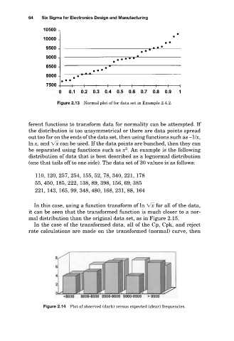
Figure 2.13 Normal plot of for data set in Example 2.4.2.

ferent functions to transform data for normality can be attempted. If
the distribution is too unsymmetrical or there are data points spread
out too far on the ends of the data set, then using functions such as –1/x,
ln x, and x can be used. If the data points are bunched, then they can
2
be separated using functions such as x . An example is the following
distribution of data that is best described as a lognormal distribution
(one that tails off to one side). The data set of 30 values is as follows:
110, 120, 257, 254, 155, 52, 78, 340, 221, 178
55, 450, 185, 222, 138, 89, 398, 156, 69, 385
221, 143, 165, 99, 348, 480, 168, 231, 88, 164

In this case, using a function transform of ln x for all of the data,
it can be seen that the transformed function is much closer to a nor-
mal distribution than the original data set, as in Figure 2.15.
In the case of the transformed data, all of the Cp, Cpk, and reject
rate calculations are made on the transformed (normal) curve, then

Figure 2.14 Plot of observed (dark) versus expected (clear) frequencies.