Page 92 - Six Sigma for electronics design and manufacturing

The Elements of Six Sigma and Their Determination

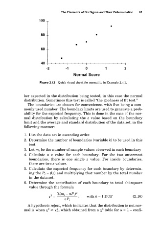
Figure 2.12 Quick visual check for normality in Example 2.4.1. 61

ber expected in the distribution being tested, in this case the normal
distribution. Sometimes this test is called “the goodness of fit test.”
The boundaries are chosen for convenience, with five being a com-
monly used number. The boundary limits are used to generate a prob-
ability for the expected frequency. This is done in the case of the nor-
mal distribution by calculating the z value based on the boundary
limit and the average and standard distribution of the data set, in the
following manner:

1. List the data set in ascending order.
2. Determine the number of boundaries (variable k) to be used in this
test.
3. Let m i be the number of sample values observed in each boundary
4. Calculate a z value for each boundary. For the two outermost
boundaries, there is one single z value. For inside boundaries,
there are two z values.
5. Calculate the expected frequency for each boundary by determin-
ing the P i = f(z) and multiplying that number by the total number
in the data set.
6. Determine the contribution of each boundary to total chi-square
value through the formula
(m i – nP i ) 2
2
= ; with k – 1 DOF (2.16)
nP i
A hypothesis reject, which indicates that the distribution is not nor-
mal is when , which obtained from a table for = 1 – confi-
2
2
2