Page 94 - Six Sigma for electronics design and manufacturing

The Elements of Six Sigma and Their Determination
63
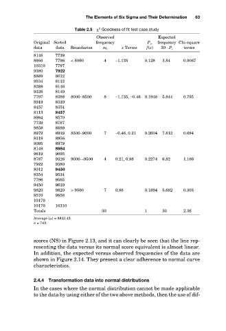
Table 2.5 Goodness of fit test case study
2
Expected
P i ,
frequency
Original Sorted
terms
data
f(z)
z Terms
30 · P i
m i
7739
8146
8956
4
0.0067
3.84
< 8000
7796
7797
10310
9380
7922
8012
8889
9534
8113
8288 data Boundaries Observed –1.135 0.128 frequency Chi-square
8146
9326 8149
7797 8288 8000–8500 8 –1.135, –0.46 0.1948 5.844 0.795
8919 8319
8457 8354
8113 8457
8984 8570
7739 8787
9858 8889
8979 8919 8500–9000 7 –0.46, 0.21 0.2604 7.812 0.084
8319 8956
9095 8979
8149 8984
9619 9095
8787 9326 9000–-9500 4 0.21, 0.88 0.2274 6.82 1.166
7922 9380
8012 9450
8354 9534
7796 9565
9450 9619
9820 9820 > 9500 7 0.88 0.1894 5.682 0.305
8570 9858
10170
10170 10310
Totals 30 1 30 2.36
Average ( ) = 8843.43.
= 743.
scores (NS) in Figure 2.13, and it can clearly be seen that the line rep-
resenting the data versus its normal score equivalent is almost linear.
In addition, the expected versus observed frequencies of the data are
shown in Figure 2.14. They present a clear adherence to normal curve
characteristics.
2.4.4 Transformation data into normal distributions
In the cases where the normal distribution cannot be made applicable
to the data by using either of the two above methods, then the use of dif-