Page 91 - Six Sigma for electronics design and manufacturing

Six Sigma for Electronics Design and Manufacturing
60
1. Randomly select a number of parts samples for measurement of
the quality characteristic, which is the part attribute of interest to
the six sigma effort. Thirty samples are considered statistically sig-
nificant. However smaller numbers might be used for a quick look
at the distribution. (For more on sample sizes, refer to Chapter 5.)
2. Rank the data in ascending order, from 1 to n.
3. Generate a normal curve score (NS) corresponding to each data
point. Each ranked data point is subtracted by 0.5, then divided by
the total number of points n so that it sits in the middle of a box of
ranked points. Each data point probability is based on the rank of
point i, with i ranging from 1 to n. The normal score (NS) repre-
sents the position of that ranked point versus its equivalent value
of the z distribution:
P(z) = (i – 0.5)/n i = 0, 1, . . . , n (2.14)
NS = z of P(z)
N = total number of parts to be checked for normality
4. Plot each data point value on the Y axis against its normal score. If
the data is normal, it should show as a straight line.
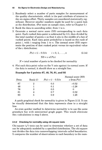
Example for 5 points: 67, 48, 76, 81, and 93
Normal score (NS)
Data Rank (i) P(z) = (i – 0.5)/n z from P(z)
67 2 0.3 –0.52
48 1 0.1 –1.28
76 3 0.5 0
81 4 0.7 0.52
93 5 0.9 1.28
A quick graphical check for normality is given in Figure 2.12. It can
be visually determined that the data represents close to a straight
line.
An even quicker method to determine normality is to use the same
procedure but with seminormal graph paper. This would eliminate
the z calculations in step 3 above.

2.4.2 Checking for normality using chi-square tests
2
Chi-square ( ) tests can be used to determine whether a set of data
can be adequately modeled by a specified distribution. The chi-square
test divides the data into nonoverlapping intervals called boundaries.
It compares the number of observations in each boundary to the num-