Page 257 - Soil and water contamination, 2nd edition

244 Soil and Water Contamination
6955

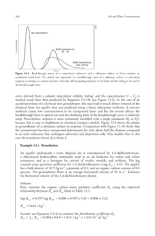
No retardation

Concentration With retardation

(R ∼ 4)

With retardation
and tailing

Time
Figure 13.3 Breakthrough curves of a conservative substance and a substance subject to linear sorption or
retardation (solid line). The dotted line represents the breakthrough curve of a substance subject to non-linear
sorption according to a convex isotherm. Note the self-sharpening tendency of the front and the tailing at the end of
the breakthrough curve.

curve derived from a column experiment exhibits ‘tailing ’ and the concentration C = C is
0
reached much later than predicted by Equation (13.10) (see Figure 13.3). In the case of an
accidental release of a chemical into groundwater, this may lead to much slower removal of the
chemical from the aquifer than was predicted using a linear adsorption isotherm. A concave
isotherm causes low concentrations to be transported faster and has the reverse effects: the
breakthrough front is spread out and the declining limb of the breakthrough curve is relatively
steep. Nevertheless, sorption is most commonly modelled with a single parameter (K or R ),
d f
because this is easy to implement in chemical transport models. Figure 13.4 shows the plume
in groundwater of a substance subject to sorption. Comparison with Figure 11.10 shows that
the contaminant has been transported downstream for only about half the distance compared
to an inert substance that undergoes advection and dispersion only. This implies that in this
case the retardation factor R is about 2.
f
Example 13.1 Retardation

An aquifer underneath a waste disposal site is contaminated by 1,4-dichlorobenzene,
a chlorinated hydrocarbon commonly used as an air freshener for toilets and refuse
containers, and as a fumigant for control of moths, moulds, and mildews. The log

octanol–water partition coefficient for 1,4-dichlorobenzene is log K = 3.43. The aquifer
ow
-3
has a bulk density of 1675 kg m , a porosity of 0.3, and an organic carbon content of 0.1
-1
percent. The groundwater flows at an average horizontal velocity of 50 m y . Estimate
the horizontal velocity of the 1,4-dichlorobenzene plume .
Solution
First, estimate the organic carbon–water partition coefficient K using the empirical

oc
relationship between K and K listed in Table 13.1:
oc ow
log K . 0 937 log K . 0 006 . 0 937 . 3 43 . 0 006 . 3 21
oc ow
K 1614 l kg -1
oc
Second, use Equation (13.4) to estimate the distribution coefficient K :

d
-1
-3
3
K f K . 0 001 1614 . 1 614 l kg = 1.614·10 m kg -1
d oc oc

10/1/2013 6:45:11 PM
Soil and Water.indd 256 10/1/2013 6:45:11 PM
Soil and Water.indd 256