Page 334 - Soil and water contamination, 2nd edition

Patterns in groundwater 321

vertical cross-sections in a shallow sandy aquifer in southern Ontario, Canada . They installed
fifteen multi-level wells down to about 3.5 m below the water table across an 11 m long
transect on an arable field perpendicular to the direction of groundwater flow. Figure 17.10
shows the observed pattern of nitrate in one of the cross-sections. Successive years of fertiliser
application can be seen as nitrate-rich zones in the cross-sections. The differences in depth
of the nitrate-rich zones originating from fertiliser application one and three years before
-1
groundwater sampling suggest a vertical groundwater flow velocity of about 0.5 m y . The
-1
horizontal groundwater flow velocity in the shallow aquifer amounts to about 50 m y . This
means that the lowest nitrate-rich band originates from fertiliser applied at about 150 m
upgradient from the cross-section.

17.6 EFFECTS OF DISPERSION

The process of dispersion tends to level out spatial differences in concentrations. In Section
11.3 we noted that given a certain concentration gradient, the magnitude of dispersion
expressed in terms of the dispersion coefficient or dispersivity depends on the scale at which
the process is studied. At the scale of contaminant plumes (spatial resolution ∼ 0.1 m),

regional scale (spatial resolution ∼ 10–100 m), or larger scales, dispersion in groundwater is
dominated by macroscopic dispersion due to heterogeneities in the hydraulic conductivity
of the sediment (Domenico and Schwarz, 1996; Zheng and Gorelick, 2003). As dispersion
is driven by the concentration gradient, it particularly brings about concentration changes
in time at locations where the concentration gradient is large: for example, at the edges of a
contaminant plume .
Contaminant concentrations are generally highest in the leachate just below the
contaminant point source . All compounds in the leachate entering the aquifer will be
diluted as the leachate mixes with the uncontaminated groundwater due to longitudinal
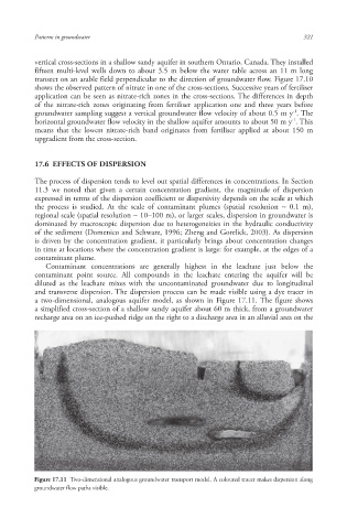
and transverse dispersion . The dispersion process can be made visible using a dye tracer in
a two-dimensional, analogous aquifer model, as shown in Figure 17.11. The figure shows
a simplified cross-section of a shallow sandy aquifer about 60 m thick, from a groundwater
recharge area on an ice-pushed ridge on the right to a discharge area in an alluvial area on the

Figure 17.11 Two-dimensional analogous groundwater transport model. A coloured tracer makes dispersion along
groundwater flow paths visible.

10/1/2013 6:47:05 PM
Soil and Water.indd 333 10/1/2013 6:47:05 PM
Soil and Water.indd 333