Page 288 - Solid Waste Analysis and Minimization a Systems Approach

266 SOLID WASTE ESTIMATION AND PREDICTION

For the general model, there are k independent variables, denoted as x , x , . . ., x k
1
2
and n observations denoted as y , y , . . ., y . Each variable is expressed by the equation
1
n
2
y = β + β x + β x + + β x + ε
i 0 1 i 1 2 i 2 k ki i

The model represents n equations describing how the dependent variables (annual
solid waste generation per company) are generated. Using matrix notation, the equations
can be written as

y = X +βε

where

β ⎡ ⎡ ⎤
y ⎡ ⎤ 1 ⎡ x x x ⎤ ⎢ 0 ⎥
⎢ 1 ⎥ ⎢ 11 21 k1 ⎥ ⎢ β 1 ⎥
y
⎢
y = ⎢ 2 ⎥ X = ⎢ 1 x 12 x 22 x k2 ⎥ β = β ⎥
⎢ ⎥ ⎢ ⎥ ⎢ 2 ⎥
⎢ ⎥ ⎢ ⎥ ⎢ ⎥
⎥
⎣ y ⎢ n ⎦ ⎣ 1 x n 1 x 2 n x kn ⎦ ⎢ ⎥
⎣ β k ⎦

The least squares solution for estimation of β involves finding β for which

SSE = (y − Xβ)′(y − Xβ)

is minimized. The minimization process involves solving β for the equation

∂
( SSE) = 0
∂b

The result reduces to the solution of β in

(X′X)β= X′y

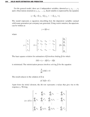
Apart from the initial element, the ith row represents x-values that give rise to the
response y . Writing
i

⎡ n n n ⎤
⎢ n ∑ x i 1 ∑ x i 2 ∑ x ki ⎥
⎢ i=1 i=1 i=1 ⎥ ⎥
⎢ n n n n ⎥
⎢ ∑ x ∑ x 2 xx ∑ x ⎥
A = X X ′ = ⎢ i=1 i 1 i=1 1i ∑ 1 i 2 i i=1 i 1 ⎥
i
i=1
⎢ ⎥
⎢ ⎥
⎢ n n n n ⎥
ki 1i ∑
⎢ ∑ x ki ∑ x x 1 xx 2i ∑ x 2 ki ⎥
ki
⎣ i=1 i= 1 i= 1 i= 1 ⎦