Page 289 - Solid Waste Analysis and Minimization a Systems Approach

STEPWISE REGRESSION METHODOLOGY 267

and

⎡ n ⎤
⎢ g = ∑ y i ⎥
0
⎢ i=1 ⎥
⎢ n ⎥
⎢ g = ∑ x y ⎥
g = X y ′ = ⎢ 1 i=1 ii ⎥
⎢ ⎥
⎢ ⎥
⎢ n ⎥
k ∑
ki i ⎥
⎢ g = x y
⎣ ⎣ i=1 ⎦

the normal equations can be put in matrix form

Aβ= g

If the matrix A is nonsingular, the solution for the regression coefficients is written as

−1
β= Ag = X ′X) −1 ′ X y
(
The regression equation is obtained by solving a set of k + 1 equations for the like
number of unknowns. This involves the inversion of k + 1 by k + 1 matrix X′X.
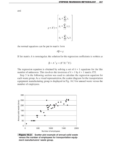
Step 3 in the following section was used to calculate the regression equation for
each waste group. As a visual representation, the scatter diagram for the transportation
equipment manufacturing group is displayed in Fig. 16.3 for annual waste versus the
number of employees.

300

250
Annual solid waste (tons) 200

150

100

50

0
0 500 1000 1500 2000
Number of employees
Figure 16.3 Scatter plot example of annual solid waste
versus the number of employees for transportation equip-
ment manufacturers’ waste group.