Page 294 - Solid Waste Analysis and Minimization a Systems Approach

272 SOLID WASTE ESTIMATION AND PREDICTION

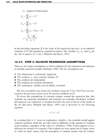
n = number of observations

xx ∑
S = n ( x − ) 2
x
i
i=1
yy ∑
S = n ( y − y) 2
i
i=1
xy ∑
S = n ( x − x y − y)
(
)
i
i
i=1
S
S − βS
s = yy xy
n − 2

In the preceding equations, β is the slope of the regression line and s is an unbiased
2
estimator of σ (the population standard deviation). The variables S , S , and S are
xx
yy
xy
the sum of squares for x and y (Walpole and Myers, 1993).

16.3.5 STEP 5: VALIDATE REGRESSION ASSUMPTIONS

There are five major assumptions or ideal conditions for the estimation and inference
in multiple regression models (Dielman, 1996). The five assumptions are

1 The relationship is statistically significant.
2 The residuals, e , have constant variance σ 2 .
i
e
3 The residuals are independent.
4 The residuals are normally distributed.
5 The explanatory variables are not highly correlated.

The first assumption was tested and validated using the F-test. The F-test was dis-
cussed in the previous section at the 95 percent confidence level.
To access the assumptions of constant variance around the regression line, that
residuals are randomly distributed, and residuals are normally distributed, residual
plot analysis was conducted. A residual describes the error in the fit of the model at
the ith data point (Walpole and Myers, 1993) and is described in the following
equation:

e = y − ˆ
y
i i i

In a residual plot of ˆ e i versus an explanatory variable x, the residuals should appear
scattered randomly about the zero line with no difference in the amount of variation
in the residuals, regardless of the value of x (Dielman, 1996). If there appears to be a
difference in variation (for example, if the residuals are more spread out for larger values
of x than for small values), then the assumption of constant variance may be violated.