Page 295 - Solid Waste Analysis and Minimization a Systems Approach

STEPWISE REGRESSION METHODOLOGY 273

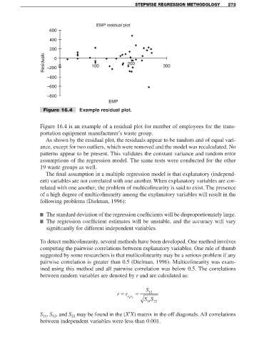
EMP residual plot
600

400

200
Residuals –200 0 100 200 300
0

–400
–600

–800
EMP
Figure 16.4 Example residual plot.

Figure 16.4 is an example of a residual plot for number of employees for the trans-
portation equipment manufacturer’s waste group.
As shown by the residual plot, the residuals appear to be random and of equal vari-
ance, except for two outliers, which were removed and the model was recalculated. No
patterns appear to be present. This validates the constant variance and random error
assumptions of the regression model. The same tests were conducted for the other
19 waste groups as well.
The final assumption in a multiple regression model is that explanatory (independ-
ent) variables are not correlated with one another. When explanatory variables are cor-
related with one another, the problem of multicolinearity is said to exist. The presence
of a high degree of multicolinearity among the explanatory variables will result in the
following problems (Dielman, 1996):

■ The standard deviation of the regression coefficients will be disproportionately large.
■ The regression coefficient estimates will be unstable, and the accuracy will vary
significantly for different independent variables.

To detect multicolinearity, several methods have been developed. One method involves
computing the pairwise correlations between explanatory variables. One rule of thumb
suggested by some researchers is that mutlicolinearity may be a serious problem if any
pairwise correlation is greater than 0.5 (Dielman, 1996). Multicolinearity was exam-
ined using this method and all pairwise correlation was below 0.5. The correlations
between random variables are denoted by r and are calculated as:

r = r = S 12
xx
SS
12
11 22
S , S , and S may be found in the (X′X) matrix in the off diagonals. All correlations
11
12
22
between independent variables were less than 0.001.