Page 145 - Statistics II for Dummies

Chapter 7: Getting Ahead of the Learning Curve with Nonlinear Regression 129

Residual Plots for Quiz Score
Normal Probability Plot of the Residuals Residuals versus the Fitted Values
99 2
90 1
Percent 50 Standardized Residual 0

10 −1
1 −2
−2 −1 0 1 2 0.0 2.5 5.0 7.5 10.0
Standardized Residual Fitted Value
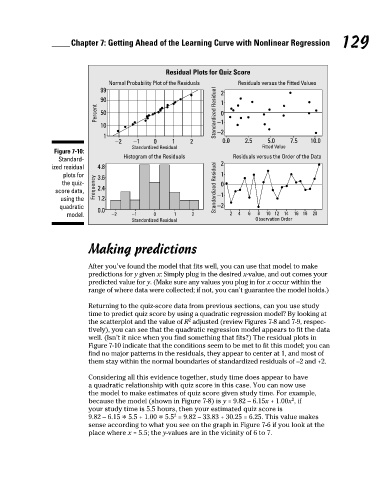
Figure 7-10:
Standard- Histogram of the Residuals Residuals versus the Order of the Data
ized residual 4.8 2
plots for 3.6 1
the quiz- 0
score data, Frequency 2.4 Standardized Residual
using the 1.2 −1
quadratic 0.0 −2
10 12 14
8
model. −2 −1 0 1 2 2 4 6 Observation Order 16 18 20
Standardized Residual

Making predictions

After you’ve found the model that fits well, you can use that model to make
predictions for y given x: Simply plug in the desired x-value, and out comes your
predicted value for y. (Make sure any values you plug in for x occur within the
range of where data were collected; if not, you can’t guarantee the model holds.)
Returning to the quiz-score data from previous sections, can you use study
time to predict quiz score by using a quadratic regression model? By looking at
the scatterplot and the value of R adjusted (review Figures 7-8 and 7-9, respec-
2
tively), you can see that the quadratic regression model appears to fit the data
well. (Isn’t it nice when you find something that fits?) The residual plots in
Figure 7-10 indicate that the conditions seem to be met to fit this model; you can
find no major patterns in the residuals, they appear to center at 1, and most of
them stay within the normal boundaries of standardized residuals of –2 and +2.

Considering all this evidence together, study time does appear to have
a quadratic relationship with quiz score in this case. You can now use
the model to make estimates of quiz score given study time. For example,
2
because the model (shown in Figure 7-8) is y = 9.82 – 6.15x + 1.00x , if
your study time is 5.5 hours, then your estimated quiz score is
2
9.82 – 6.15 * 5.5 + 1.00 * 5.5 = 9.82 – 33.83 + 30.25 = 6.25. This value makes
sense according to what you see on the graph in Figure 7-6 if you look at the
place where x = 5.5; the y-values are in the vicinity of 6 to 7.

12_466469-ch07.indd 129 7/24/09 9:39:10 AM