Page 117 - Statistics and Data Analysis in Geology

Analysis of Sequences of Data

X
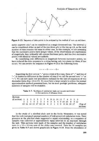
Figure 4-13. Sequence of data points to be analyzed by the method of runs up and down.

entire segment cdef can be considered as a single downward run. The interval ij
can be considered either as part of the run down ghi or the run up ijk, as the total
number of runs remains the same in either case. In this example, we are assuming
that the successive points have integer values. If the observations are expressions
of magnitude, they ordinarily will contain fractional parts, and ties (two successive
points with identical values) are unlikely.
By considering only differences in magnitude between successive points, we
have reduced the data sequence to a string having only two states (or three, if ties
occur). We can rewrite the sequence in Figure 4-13 in the following form:

+ + + -0- + - -o+

Regarding the first zero as ‘I-” gives a total of five runs, three of “+” and two of
‘I-” (it makes no difference in the number of runs if we call the second zero “+” or
“-”). We can now apply test procedures outlined for the case of sequences of two
dissimilar items (Eqs. 4.8-4.10). We must have a large sample to utilize the normal
approximation method presented here, but in most geologic problems, adequate
numbers of samples will be available.

Table 4-7. Numbers of radiolarian tests per square centimeter
in thin sections of siliceous shale.
(Bottom
ofsection) 1 2 3 2 3 5 7 9 9 11 10 12 7 4 3 2 3
2 2 1 0 2 3 2 0 3 3 491010 8 912
10 12 14 22 17 19 14 4 2 1 0 0 8 14 16 27 (Topof
section)

In the study of a silicified shale unit in the Rocky Mountains, it was noted
that the rock contained unusual numbers of well-preserved radiolarian tests. Their
presence in the silicified shale suggested a causal relationship, so a sequence of
samples was collected at approximately equal intervals in an exposure through
the unit. Thin sections were made of the samples and the number of radiolarian
tests in a 10 x 10-mm area of the slides was counted. Data for 50 samples are
given in Table 4-7 and shown graphically in Figure 4-14. Does the abundance of

189