Page 112 - Statistics and Data Analysis in Geology

Statistics and Data Analysis in Geology - Chapter 4

be developed later in this chapter, we can conclude that the events are occurring
independently in time or space.
If we have established that the series is neither autocorrelated nor contains a
trend, we may wish to test the possibility that the events are distributed accord-
ing to a Poisson distribution. You will recall from Chapter 2 that the Poisson is
a discrete probability distribution that can be regarded as the limiting case of the
binomial when n, the number of trials, becomes very large, and p, the probability
of success on any one trial, becomes very small. We can imagine that our time
series is subdivided into n intervals of equal duration. If events occur randomly,
the number of intervals that contain exactly 0, 1, 2,. . . , x events will follow the bi-
nomial distribution. As we make the lengths of the intervals progressively shorter,
n becomes progressively larger and the probabilities of occurrence decline. The
binomial distribution becomes difficult to compute, but the Poisson can be readily
used because it does not require either n or p directly. Instead, the product np = h
is all that is needed, which is given by the rate of occurrence of events.
The Poisson probability model assumes that (a) the events occur independently,
(b) the probability that an event occurs does not change with time, (c) the proba-
bility that an event will occur in an interval is proportional to the length of the
interval, and (d) the probability of more than one event occurring at the same time
is vanishingly small.
The equation for the Poisson distribution in this instance is

p(X) = e-”AX/X! (4.6)

Note that the rate of occurrence, A, is the only parameter of the distribution. Typ-
ical Poisson frequency distributions are shown in Figure 4-12. The distribution is
applicable to such problems as the rate that telephone calls come to a switchboard
or the length of time between failures in a computer system. It seems reasonable
that it also may apply to the series of geological events described at the beginning
of this section. If we can determine that our series follows a Poisson distribution,
we can use the characteristics of the distribution to make probabilistic forecasts of
the series.
The Kolmogorov-Smirnov test provides a simple way to test the goodness of fit
of a series of events to that expected from a Poisson distribution. First, the series
must be converted to a cumulative form
ti
yi = -
T
where ti is the time from the start of the series to the ith event, and T is the total
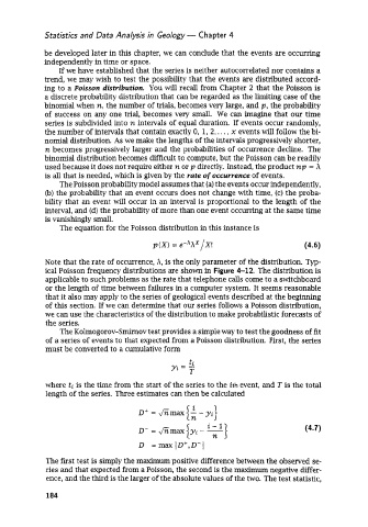
length of the series. Three estimates can then be calculated

The first test is simply the maximum positive difference between the observed se-
ries and that expected from a Poisson, the second is the maximum negative differ-
ence, and the third is the larger of the absolute values of the two. The test statistic,

184