Page 118 - Statistics for Environmental Engineers

L1592_Frame_C13.fm Page 114 Tuesday, December 18, 2001 1:49 PM

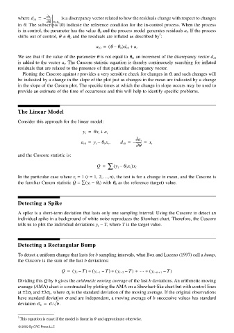
where d t0 = – ∂a t is a discrepancy vector related to how the residuals change with respect to changes
------
∂θ θ=θ 0
in θ. The subscripts (0) indicate the reference condition for the in-control process. When the process
is in control, the parameter has the value θ 0 and the process model generates residuals a t . If the process
1
shifts out of control, θ ≠ θ 0 and the residuals are inflated as described by :
a t0 = ( θθ 0 )d t0 + a t
–
We see that if the value of the parameter θ is not equal to θ 0 , an increment of the discrepancy vector d t0
is added to the vector a t . The Cuscore statistic equation is thereby continuously searching for inflated
residuals that are related to the presence of that particular discrepancy vector.
Plotting the Cuscore against t provides a very sensitive check for changes in θ, and such changes will
be indicated by a change in the slope of the plot just as changes in the mean are indicated by a change
in the slope of the Cusum plot. The specific times at which the change in slope occurs may be used to
provide an estimate of the time of occurrence and this will help to identify specific problems.

The Linear Model

Consider this approach for the linear model:
y t = θx t + a t

a t0 = y t – θ 0 x t , d t0 = – ------- =
∂a t
∂θ x t
and the Cuscore statistic is:

Q = ∑ ( y t – θ 0 x t )x t

In the particular case where x t = 1 (t = 1, 2,…, n), the test is for a change in mean, and the Cuscore is
the familiar Cusum statistic Q = ∑(y t − θ 0 ) with θ 0 as the reference (target) value.

Detecting a Spike

A spike is a short-term deviation that lasts only one sampling interval. Using the Cuscore to detect an
individual spike in a background of white noise reproduces the Shewhart chart. Therefore, the Cuscore
tells us to plot the individual deviations y t − T, where T is the target value.

Detecting a Rectangular Bump
To detect a uniform change that lasts for b sampling intervals, what Box and Luceno (1997) call a bump,
the Cuscore is the sum of the last b deviations:
Q = ( y t – ) + ( y t−1 – ) + ( y t−2 – ) + … + ( y t−b 1+ – )
T
T
T
T
Dividing this Q by b gives the arithmetic moving average of the last b deviations. An arithmetic moving
average (AMA) chart is constructed by plotting the AMA on a Shewhart-like chart but with control lines
at ±2σ b and ±3σ b , where σ b is the standard deviation of the moving average. If the original observations
have standard deviation σ and are independent, a moving average of b successive values has standard
deviation σ b = σ/ . b

1
This equation is exact if the model is linear in θ and approximate otherwise.
© 2002 By CRC Press LLC