Page 120 - Statistics for Environmental Engineers

L1592_Frame_C13.fm Page 116 Tuesday, December 18, 2001 1:49 PM

sine component is:
Q = ∑ ( y t – )sin ( 2πt/p)
T
For a sine wave of period p = 12, the plotted Cuscore is:
Q = ∑ ( y t – )sin ( 2πt/12)
T
Notice that the amplitude of the sine wave is irrelevant.

Change in the Parameter of a Time Series Model

It was stated that process drift is a normal feature in most real processes. Drift causes serial correlation in
subsequent observations. Time series models are used to describe this kind of data. To this point, serial
correlation has been mentioned briefly, but not explained, and time series models have not been introduced.
Nevertheless, to show the wonderful generality of the Cuscore principles, a short section about time series
is inserted here. The material comes from Box and Luceno (1997). The essence of the idea is in the next
two paragraphs and Figure 13.2, which require no special knowledge of time series analysis.
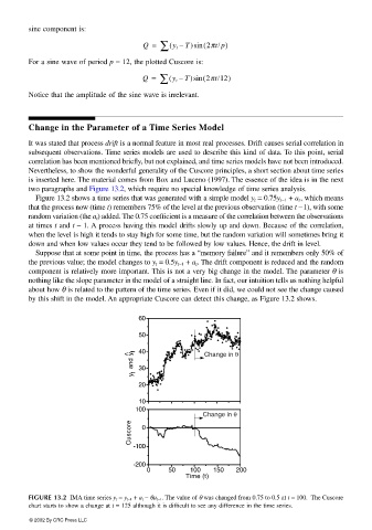
Figure 13.2 shows a time series that was generated with a simple model y t = 0.75y t−1 + a t , which means
that the process now (time t) remembers 75% of the level at the previous observation (time t − 1), with some
random variation (the a t ) added. The 0.75 coefficient is a measure of the correlation between the observations
at times t and t – 1. A process having this model drifts slowly up and down. Because of the correlation,
when the level is high it tends to stay high for some time, but the random variation will sometimes bring it
down and when low values occur they tend to be followed by low values. Hence, the drift in level.
Suppose that at some point in time, the process has a “memory failure” and it remembers only 50% of
the previous value; the model changes to y t = 0.5y t−1 + a t . The drift component is reduced and the random
component is relatively more important. This is not a very big change in the model. The parameter θ is
nothing like the slope parameter in the model of a straight line. In fact, our intuition tells us nothing helpful
about how θ is related to the pattern of the time series. Even if it did, we could not see the change caused
by this shift in the model. An appropriate Cuscore can detect this change, as Figure 13.2 shows.

60
50

y t > 40 Change in θ

and 30
y t
20

10
100
Change in θ

Cuscore 0
-100

-200
0 50 100 150 200
Time (t)

FIGURE 13.2 IMA time series y t = y t−1 + a t − θa t−1 . The value of θ was changed from 0.75 to 0.5 at t = 100. The Cuscore
chart starts to show a change at t = 125 although it is difficult to see any difference in the time series.
© 2002 By CRC Press LLC