Page 127 - Statistics for Environmental Engineers

L1592_frame_C14 Page 123 Tuesday, December 18, 2001 1:49 PM

with ν = 19 + 13 = 32 degrees of freedom. The pooled standard deviation is:

s pooled = 0.70 µg/L

The appropriate t statistic is t 32,0.01 = 2.457 and MDL = 2.457s pooled = 2.457 0.70) = 1.7µg/L .
(

An Alternate Model for the MDL
The purpose of giving an alternate model is to explain the sources of variation that affect the measure-
ments used to calculate the MDL. Certified laboratories are obliged to follow EPA-approved methods,
and this is not an officially accepted alternative.
Pallesen (1985) defined the limit of detection as “the smallest value of analyte that can be reliably
detected above the random background noise present in the analysis of blanks.” The MDL is defined in
terms of the background noise of the analytical procedure for the matrix being analyzed. The variance
of the analytical error and background noise are considered separately. Also, the variance of the analytical
error can increase as the analyte concentration increases.
The error structure in the range where limit of detection considerations are relevant is assumed to be:

y i = η + e i = η + a i + b i

The a i and b i are two kinds of random error that affect the measurements. a i is random analytical error
and b i is background noise. The total random error is the sum of these two component errors: e i = a i + b i .
Both errors are assumed to be randomly and normally distributed with mean zero.
2
Background noise (b i ) exists even in blank measurements and has constant variance, σ b . The mea-
surement error in the analytical signal (a i ) is assumed to be proportional to the measurement signal, η.
That is, σ a = κη and the variance σ a = κ η . Under this assumption, the total error variance ( ) of any
2
2
2
2
σ e
measurement is:
2
σ e = σ b + σ a = σ b + κ η .
2
2
2
2
2
2 2
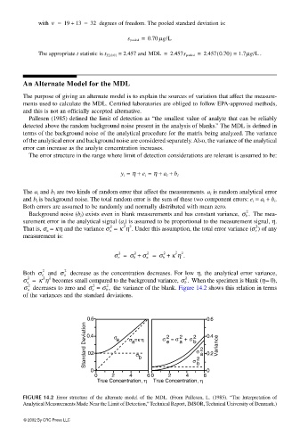
Both σ e and σ a decrease as the concentration decreases. For low η, the analytical error variance,
σ a = κ η 2 becomes small compared to the background variance, σ b . When the specimen is blank (η = 0),
2
2
2
2 decreases to zero and σ e = 2
2
σ a σ b , the variance of the blank. Figure 14.2 shows this relation in terms
of the variances and the standard deviations.
0.6 0.6
Standard Deviation 0.4 σ e σ = κη σ 2 e = σ 2 + σ 2 b σ 2 a 0.2 Variance
0.4
a
a
0.2
σ
b
b
0 σ 2 0
0 2 4 6 0 2 4 6
True Concentration, η True Concentration, η
FIGURE 14.2 Error structure of the alternate model of the MDL. (From Pallesen, L. (1985). “The Interpretation of
Analytical Measurements Made Near the Limit of Detection,” Technical Report, IMSOR, Technical University of Denmark.)
© 2002 By CRC Press LLC