Page 128 - Statistics for Environmental Engineers

L1592_frame_C14 Page 124 Tuesday, December 18, 2001 1:49 PM

The detection limit is the smallest value of y for which the hypothesis that η = 0 cannot be rejected
with some stated level of confidence. If y > MDL, it is very improbable that η = 0 and it would be
concluded that the analyte of interest has been detected. If y < MDL, we cannot say with confidence
that the analyte of interest has been detected.
Assuming that y, in the absence of analyte, is normally distributed with mean zero and variance, the
MDL as a multiple of the background noise, σ b :
MDL = z α σ b

where z α is chosen such that the probability of y being greater than MDL is (1 – α)100% (Pallesen,
1985). The probability that a blank specimen gives y > MDL is α100%. Values of z α can be found in a
table of the normal distribution, where α is the area under the tail of the distribution that lies above z a .
For example:
α = 0.05 0.023 0.01 0.0013
1.63 2.00 2.33 3.00
z a
Using z = 3.00 (α = 0.0013) means that observing y > MDL justifies a conclusion that η is not zero at
a confidence level of 99.87%. Using this MDL repeatedly, just a little over one in one thousand (0.13%)
of true blank specimens will be misjudged as positive determinations. (Note that the EPA definition is
based on t α instead of z α , and chooses α so the confidence level is 99%.)
2 2
The replicate lead measurements in Table 14.1 will be used to estimate the parameters σ b and κ in
the model:
σ e = σ b + σ a = σ b + κ η 2
2
2
2
2
2
2 2 2 2
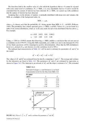
The values of σ e and η are estimated from the data by computing s e and y . The average and variance
2 2
for the laboratory are listed in Table 14.3. The parameters σ b and κ are estimated by regression, as
2 2
shown in Figure 14.3. The intercept is an estimate of σ b and the slope is estimate of κ . The estimated
TABLE 14.3
2
Estimated Averages ( ) and Variances ( ) at Each
y
s e
Concentration Level for the Data from Table 14.1
Pb Added
2
( µµ µµg/L) y s e
0 2.73 0.38
1.25 3.07 0.55
2.5 4.16 0.41
5.0 5.08 0.70
10.0 11.46 2.42
3
Laboratory B
2 2
s = 0.267 + 0.016 y
2 e
2
s e
1

0
0 50 2 100 150
y

2 2 2 2

FIGURE 14.3 Plots of s e vs. y used to estimate the parameters κ and σ b .
© 2002 By CRC Press LLC